You can download the datasets and R code file for this session here.

R Introduction

What is R
R Studio
R Environment
R Basics operations
R Packages
R Datatypes
R Scripts and Saving the work
My First R Program
R Functions
Most common errors in R
R- Help

Introduction

A programming language for data manipulations, statistical computing and graphics
R is a fairly easy language to learn.
By knowing some essential basics we can get started with data analytics.
Later on, we can build our r coding capability by learning while working
A good learning path for getting started in any data analysis tool or language contains 3 major steps
Basics, environment, coding syntax
Data handling
Important functions and Performing analysis

What is R

A programming language for data manipulations, statistical computing and graphics
Programming “environment”
Open source
Contains numerous statistical methods
Excellent graphics capabilities
Supported by a large user network
R contains some statistical algorithms that are not yet available in other tools
Mostly considered as language than a tool

R- A Comprehensive Analytical Tool

Can connect to any type of database
Oracle, ODBC, Microsoft Excel, PostgreSQL, MySQL, SPSS, Oracle Data Miner, SAS/IML, JMP, Pentaho Kettle, Jaspersoft BI, SAP HANA and Hadoop
Super visualization and graphics capabilities
Numerus dedicated packages/ libraries for visualizations.
Availability of all statistical algorithms
Most of the research scholars use R in their course work. Hence most of the algorithms are available
Many more solutions
Data Handling, Data mining , data visualization, text mining, Big data & Machine learning

Download and Install R

Go to the R homepage and locate the download link http://cran.r-project.org/
Select the relevant version & download it
Install it by executing the .exe file

R-Studio

R studio is an user-friendly UI for interacting with R
R is command line interface, coding might be little slow for learners
Where as R studio gives us shortcuts for direct clicks
It is a free and open-source integrated development environment (IDE) for R
R studio has comprehensive abilities to make the coding on R more efficient
You need R to make R-Studio work
R-Studio is just a skin, the actual core programming language is R. All the commands typed in R-Studio will be submitted to R and the output will be fetched and displayed in R Studio

Download and Install R-Studio

Go to the R-Studio homepage and locate the download link https://www.rstudio.com/
Select the relevant version & download it
Install it by executing the .exe file

Three Main Windows

Console
Workspace
Output

R Console

This is where we type and submit the commands
Most of the times the output is shown in the console itself
Hit Enter key to submit the commands
Up and Down arrows will recall previous command
Type partial command and use ‘tab’ key for autofill recommendations

R – Quick Warm-up

68+28

## [1] 96

134*456

## [1] 61104

sqrt(119)

## [1] 10.90871

log(10)

## [1] 2.302585

exp(5)

## [1] 148.4132

Workspace

During an R session, all user defined objects are stored in a temporary, working memory
Commands are entered interactively at the R user prompt.
Up and down arrow keys scroll through your command history.
list objects ls()
remove objects rm()
data()
The objects in the workspace will last for just for that session, unless we save the workspace

The Assign Operator

“<-” used to indicate assignment

x<-7

y<-68+28

z<-134*456

k<-sqrt(119)

Assignment to an object is denoted by “<-” or “->” or “=”.

Naming convention

Must start with a letter (A-Z or a-z)
Can contain letters, digits (0-9), and/or periods “.”
R is a case sensitive language.
newdata different from NewData

LAB: Working with R

x <- rnorm(1000,mean=20,sd=5) 
x

##    [1] 29.727512 22.027772 14.173818 11.567661 11.290773 28.545150
##    [7] 23.336270 10.623532 25.238777 28.339100 19.317402 22.607638
##   [13] 16.696072 20.682688 18.952773 21.853967 24.366763 19.695094
##   [19] 17.400101 21.136721 29.736818 23.917742 25.168942 25.422684
##   [25] 11.653086 22.272998 27.392081 15.312394 20.621272 20.774217
##   [31] 26.400664 20.912214 21.110055 24.317066 18.775163 19.759073
##   [37] 17.423549 25.615045 20.155949 20.382279 24.729653 17.432053
##   [43] 17.433073 16.289813 22.945870 24.711526 17.996536 17.654353
##   [49] 33.622504 17.235110 24.032638 18.196793 14.204424 15.881424
##   [55] 20.831512 29.730846 19.276928 18.181224 25.362097 14.644336
##   [61] 22.779562 11.467166 17.549835 22.901572 30.653036 13.740296
##   [67] 15.412779 21.977330 26.986697 23.066531 20.802516 27.602665
##   [73] 21.174894 19.420062 29.804671 25.722596 22.245351 20.137828
##   [79]  8.641546 18.413145 16.674934 17.744648 14.345363 26.419367
##   [85] 25.286868 22.819012 19.278091 24.047195 20.367724  7.406066
##   [91] 25.085621 24.219120 19.048239 22.182127 10.387633 26.160024
##   [97] 21.120116 20.110008 26.169600 21.986982 23.216666 28.166575
##  [103] 17.877387 12.994729 13.082539 19.386388 21.613470 26.454635
##  [109] 21.686849 27.967669 14.250426 19.472040 17.442288 15.332908
##  [115] 27.594943 28.256114 32.458636 16.783834 14.985155 25.150545
##  [121] 12.632237 16.698488 11.660866 21.716199 20.933646 22.702097
##  [127] 15.476770 20.205206 26.343377 10.139146 15.813740 15.634903
##  [133] 16.514700 24.291489 15.913789 23.240543 20.506762 16.580606
##  [139] 22.207518  9.691391 16.676488 19.984987 21.002244 17.029171
##  [145] 20.806644 11.498186 19.899529 22.933672 14.163869 21.947553
##  [151] 25.157130 18.244896 16.461983  8.412688 25.306571 23.125001
##  [157] 17.606258 30.266219 22.116809 16.431025 17.083604 15.466805
##  [163] 24.401583 19.544583 19.942909 27.119469 18.213193 14.463331
##  [169] 22.176626 19.306320 17.776627 22.418411 17.234031 18.643855
##  [175] 14.138607 24.799317 13.090200 21.463304 34.173550 16.199937
##  [181] 17.352828 28.606000 15.466058 18.753820 25.505661 22.614690
##  [187] 27.898874 24.758957 18.805842 20.594374 22.588168 23.769131
##  [193] 19.655519  9.011509 25.684415 20.046036 16.952598 29.516783
##  [199] 20.608292 15.339981 25.789671 21.119468 15.386253 17.075294
##  [205] 20.530112 17.378699 22.577657 23.077779 16.267017 34.587203
##  [211] 17.038457 22.662198 18.369485 20.938257 17.675383 16.516821
##  [217] 19.366059 12.921027 21.492170 19.151660 28.779073 15.795389
##  [223] 22.036802 26.010214 18.312752 16.922768 19.836704 23.957549
##  [229]  8.068545 20.327931 15.564294 31.962241 12.362306 24.442804
##  [235] 22.079282 22.009864 30.348366 16.951518 17.823881 13.821275
##  [241] 23.030961 23.299950 17.091296 13.137487 17.041698 19.996918
##  [247] 20.373975 32.081578 23.157645 17.717973 19.656141 19.713430
##  [253] 16.304237 15.845531 21.181814 18.263276 31.491360 13.226387
##  [259] 20.753108 33.975560 21.556913 25.103936 30.089965 10.538623
##  [265] 30.962363 23.459218 13.792790 19.196656 20.129247 24.564201
##  [271] 24.577835 21.519863 29.632636 13.814721 25.846305 29.057134
##  [277] 20.171712 18.640709 26.183392 16.849311 13.704763 20.029619
##  [283] 16.997223 25.276494 25.027250 15.552910 27.133327 23.615325
##  [289] 25.210040 18.196115 16.591711 16.425250 15.852650 16.721285
##  [295] 23.976945 23.120209 16.552743 22.714420 22.319958 31.019111
##  [301] 23.850647 17.985637 21.325981 23.062039 17.563887 13.274493
##  [307] 13.466433 19.765545 11.638812 21.977456 31.443411 19.689766
##  [313] 19.683234 22.671269 27.047825 21.140776 14.350831 23.163323
##  [319] 24.993487 13.308481 17.804535 17.430428 22.258972 16.858152
##  [325] 24.146135 28.916969 20.784642 22.103654 23.235227 18.363599
##  [331] 17.491072 22.285308 27.187974 24.384006 25.319820 25.645659
##  [337] 18.077088 15.741573 17.156785 17.726549 15.399142 22.906717
##  [343] 26.668604 20.498866 30.550796 22.255092 21.430002 17.090993
##  [349] 21.083509 26.410319 25.184856  7.431343 22.397728 18.231511
##  [355] 23.770490 22.288674 21.518100 17.622687 20.853831 16.578927
##  [361] 23.623828 15.994951 30.322290 20.969471 18.448244 20.520756
##  [367] 19.460768 21.296014 18.290777 15.212567 26.234917 17.666005
##  [373] 23.687114 26.716202 13.969268 24.962188 23.602565 14.667628
##  [379] 23.822215 18.320073 19.108169 17.859525 17.757073 25.693470
##  [385] 21.641692 17.674582 13.870166 12.694512 19.477806 22.126312
##  [391] 21.341572 15.989978 28.426667 16.442703 26.313395 11.106016
##  [397] 21.517167 19.037988 32.208319 21.036600 10.401488 31.509901
##  [403] 16.909775 18.415838  9.804727 22.178392 13.978888 24.746192
##  [409] 14.801578 17.466264 18.272845 19.615796 21.026918 26.233214
##  [415] 20.083827 22.525222  9.372677  5.471432 16.726941 19.586206
##  [421] 22.416402 15.593327 23.508801 22.653192 21.768656 21.190214
##  [427] 29.530999  7.345017 20.875496 12.102681 22.081654 25.687963
##  [433] 10.674088 21.643438 21.733889 21.527027 29.696669 19.753639
##  [439] 22.414899 17.257994 13.960491 30.577455 13.590040 16.520321
##  [445] 20.385122 23.055598 13.264064 13.384380 26.204026 15.962176
##  [451] 30.001610 24.975408 22.229407 25.832827 20.740921 17.902771
##  [457] 16.818382 20.727127 18.295186 13.015456 17.720566 23.635101
##  [463] 24.290884 19.195902 14.333086 16.042536 21.576213 22.272675
##  [469] 17.318944 30.251992 18.554159 29.921826 23.126921 22.335424
##  [475] 11.337965  9.712197  8.717392 15.707144 29.278814 19.281417
##  [481] 18.233900 12.032921 18.732276 16.491830 15.407045 24.378203
##  [487] 17.095985 21.029514 16.466080 19.070435 15.672621 18.779453
##  [493] 22.927014 26.485272 22.902771 21.741249 24.942199 22.276011
##  [499] 19.850424 15.324483 19.433889 18.308885 26.614344 21.896915
##  [505] 11.770512 25.121654 18.051333 25.562428 28.974449 21.074008
##  [511] 24.134702  8.458984 20.923043 25.735673 20.900147 14.571439
##  [517] 23.795236 11.557096 19.032457 29.499164 19.420786 21.199031
##  [523] 25.932573  8.876581 12.821955 18.202377 18.554885 23.426905
##  [529] 26.536813 21.380011 21.846392 16.335892 24.277272 28.138421
##  [535] 26.500791 23.818051 11.960563 23.589115 19.475901 18.853133
##  [541] 21.214499 28.666910 24.947389 17.659138 12.469256 27.073906
##  [547] 26.686557 23.085566 14.240169 14.808822 16.688735 13.946308
##  [553] 27.804613 27.700073 15.900484 18.888252 23.150262 20.993335
##  [559] 20.078851 23.775798 26.474347 14.854370 20.240155 24.757675
##  [565] 22.219904 16.192665 13.060905 26.078641 17.518245 25.785360
##  [571] 28.437244 16.988412 20.572044 16.155074 24.252410 20.858714
##  [577] 22.430396 26.036905 11.690045 12.464086 30.407987 31.106195
##  [583] 15.477675 19.804692 19.451855 22.531757 22.320660 17.879739
##  [589] 34.887069 22.801761 21.179131 14.492035 28.361927 29.077376
##  [595] 20.534770 26.247919 20.395065 21.099368  9.295359 21.247362
##  [601] 10.408193 18.622757 25.963462 27.524196 22.760837 17.005384
##  [607] 22.010480 25.358175 21.348835 20.721979 14.261099 26.914990
##  [613] 21.060421 17.496182 20.226238 27.610966 22.209560 20.015765
##  [619] 16.287719 12.893625 26.409264 14.567679 29.352838 19.716488
##  [625] 22.001347 17.045938 12.300877 19.785634 19.221634 16.768579
##  [631] 13.309049 22.909324 24.992536 15.502990 20.884396 22.417801
##  [637] 15.081900 21.522051 24.911567 24.561802 19.743491 17.364330
##  [643] 11.448953 24.816523 15.493115 21.037278 22.436472 14.611121
##  [649] 24.101681 16.471575 23.441284 20.519828 14.437120 21.932926
##  [655] 25.019366 21.190071 21.717150 23.081726 20.684399 19.836137
##  [661] 15.419452 21.184117 26.328972 20.669426 16.886217 16.478219
##  [667] 23.762737 29.938412 15.331936 10.079235 18.091092 12.324329
##  [673] 19.437112 19.931701 25.508238 21.073580 23.088567 18.154038
##  [679] 17.463793 25.977010 29.278583 23.100171 25.379744 21.772949
##  [685] 16.971225 20.761156 12.820146 30.591575 20.839551 31.781976
##  [691] 15.987095 17.504043 28.677303 16.711454 15.792376 18.828107
##  [697] 22.164995 17.282692 19.343596 22.531538 20.263012 19.678264
##  [703] 18.709399 20.405853 20.782477 19.767363 16.053323 27.061384
##  [709] 19.737181 26.483659 19.398232 22.890951 12.145002 26.302212
##  [715] 20.752499 12.414235 23.207896 30.764119 27.088660 13.567575
##  [721] 13.596255 25.377880 24.870826 17.340803 24.755759 25.542423
##  [727] 19.115129 21.414287 23.440763 27.871175 22.037819 23.180335
##  [733] 22.511037 19.221952 15.939205 25.054925 30.220672 13.119708
##  [739] 15.706674 25.004249 19.257284 16.632356 19.541559 16.974871
##  [745] 16.852292 24.538191 23.413720 22.405756 17.476713 18.778854
##  [751] 20.829434 19.111266 24.626245 24.301301 21.936837 21.610876
##  [757] 23.844085 30.350177 21.518825 19.280792 23.284695 26.628839
##  [763] 24.106712 19.448038 14.513543 20.719627 26.996327 14.628779
##  [769] 22.572400 10.394729 17.961564 23.135872 15.984582 24.298295
##  [775] 19.188606 21.169912 17.830440 25.480069 14.568884 15.680531
##  [781] 19.830539 18.630551 20.866931 27.819166 15.121630 13.843840
##  [787] 16.388020 17.040887 19.785344 16.278083 22.651521 24.395421
##  [793] 25.486104 25.549499 22.980868 19.648534 14.658246 12.985290
##  [799] 27.238426 22.086507 15.030376 26.842067 18.007588 22.657393
##  [805] 28.744461 24.935354 17.174687 18.403790 23.801563 27.410771
##  [811] 14.474528 23.857910 18.500923 20.949005 16.417592 23.272319
##  [817] 13.074286 12.346769 23.483140 20.184164 18.510095 22.052894
##  [823] 20.589209 25.118588 26.846245 22.489599 25.267335 12.491648
##  [829] 19.373453 16.047960 18.556984 16.257403 21.905341 20.213579
##  [835] 16.548013 12.471732 25.618366 28.437215 17.456180 18.373999
##  [841] 17.881439 17.545000 25.063343 24.855744 12.930833 23.838372
##  [847] 17.539595 15.891848 21.157843 20.735751 18.970610 16.890390
##  [853] 15.906976 23.509515 20.399574 18.058508 21.689823 22.778539
##  [859] 22.723346 21.015544 21.295720 16.465603 13.611244 16.586355
##  [865] 20.908675 21.148464 26.357688 18.260495 16.272430 16.755129
##  [871] 25.984127 31.489427 17.261744 21.772685 22.007434 24.851916
##  [877] 19.733491 20.589950 14.416504 21.628835 23.928860 10.147253
##  [883] 16.553029 14.502338 21.434648 21.507492 15.579007 22.270235
##  [889] 19.189912 22.075889 23.655799 17.971290 25.127437  7.930384
##  [895] 19.048262 17.705362 14.745877 19.528426 30.919585 19.000064
##  [901] 19.304166 19.775426 17.546814 19.157778 13.854038 16.572636
##  [907] 16.745860 20.939633 12.698834 17.521182 18.247028 15.698520
##  [913] 16.377031 21.862080 22.000891 20.879660 13.626218 23.695772
##  [919]  9.929162 25.062728 14.243576 13.266657 10.237104 17.133295
##  [925] 14.053217 15.329687 12.266174 22.342217 13.786468 20.427231
##  [931] 20.518508 15.643824 16.700909 23.960381 17.542203 11.539881
##  [937] 14.208695 22.459240 22.399263 11.164244 33.942188 24.081148
##  [943] 25.887615 23.564897 20.836841 27.789659 23.848107 19.531269
##  [949] 20.795473 16.967840 20.019288 17.733159 13.076931 14.758359
##  [955] 15.186519 13.594224 17.271994 14.996255 18.831467 31.342821
##  [961] 23.492658 22.039948 21.045584 23.673465 16.381956  9.372736
##  [967] 20.180343 20.821498 19.630436 20.919515 19.234222 27.355534
##  [973] 21.447976 21.647215 19.309875 26.374084 25.485520 17.149242
##  [979] 15.161896 15.295486 11.753244 21.928955 18.138346 21.055981
##  [985] 19.484901 16.884938 27.356565 27.056626 13.589372 19.441235
##  [991] 25.480919 14.468213 35.919713 19.517106 11.803202 10.565383
##  [997] 17.919860 23.029789 20.178839 24.005591

mean(x)

## [1] 20.313

m <- mean(x)
m

## [1] 20.313

s<-sd(x)
s

## [1] 5.044078

R Packages

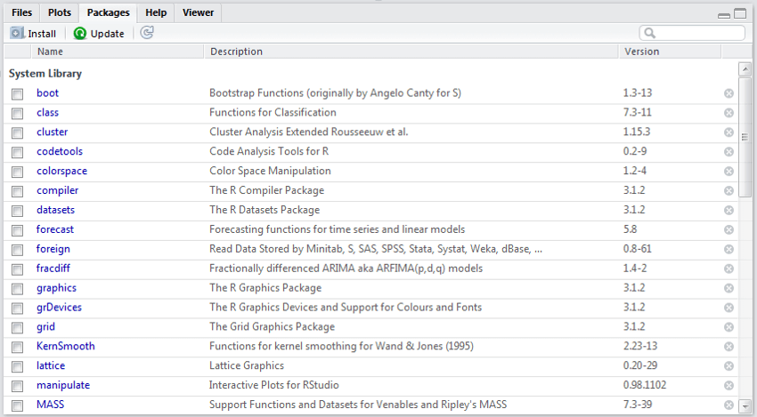
R consists of a core and packages. Packages contain functions that are not available in the core.
Collections of R functions, data, and compiled code
When you download R, already a number (around 30) of packages are downloaded as well.
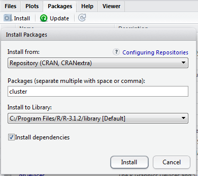
Select the ‘Packages’ menu and select ‘Install Package’, a list of available packages on your system will be displayed.
Select one and click ‘OK’, the package is now attached to your current R session. Via the library function
Before using a function, we need to install the package that contains it

Download & Install Package

Load a package

LAB: Installing packages

Create three random vectors x, y, z of size 1000.
Use rnorm() function to create these vectors.
Draw a 3d scatter plot of these three vectors use the code scatterplot3d(x,y,z)

Code: Installing packages

x <- rnorm(1000,mean=20,sd=5) 
y <- rnorm(1000,mean=15,sd=3) 
z <- rnorm(1000,mean=25,sd=8) 


install.packages("scatterplot3d", repos = 'cran.rstudio.com')
library(scatterplot3d)
scatterplot3d(x,y,z)

Some Useful Packages in R

There are nearly 7000 packages in R
Data handling Packages:
RODBC,RMySQL,RPostgresSQL,RSQLite, downloader, XLConnect,xlsx, foreign, dplyr, tidyr, plyr, reshape2, zoo
Data visualization packages:
ggplot2,ggvis, rgl, htmlwidgets, dygraphs, plotly, shiny, rcdimple
Advanced Analysis Packages:
Car, mgcv, lme4/nlme, randomForest, multcomp, vcd, glmnet, survival, e1071, Forecast, nnet

R- Data Types

Vectors
Basic R Type.
Data Frames
Collection of vectors.
Lists
Collection of R objects
Other type
Matrix
Factor
Array

R Vectors

The basic data structure in R is the vector.
Vectors are the simplest R objects, an ordered list of primitive R objects of a given type (e.g. real numbers, strings and logical).
Vectors are indexed by integers starting at 1
You can create a vector using the c() function which concatenates some elements

R Vectors

name <-'March'
is.vector(name)

## [1] TRUE

Age<-29
is.vector(Age)

## [1] TRUE

c() is a concatenate operator

Age <- c(15, 17, 16, 15, 16)
English<- c(40, 56, 30, 68, 35)
Science<- c(85, 80, 74, 39, 65)
Name<- c("John", "Bob", "Kevin", "Smith", "Rick")

is.vector(Age)

## [1] TRUE

is.vector(English)

## [1] TRUE

is.vector(Name)

## [1] TRUE

Most mathematical functions and operators can be applied to vectors without writing any loops

Age+3

## [1] 18 20 19 18 19

English1<- English+10
English1<-80
Total<- English1 + Science 
Total

## [1] 165 160 154 119 145

Age/Total

## [1] 0.09090909 0.10625000 0.10389610 0.12605042 0.11034483

Accessing Vector Elements

Use the [] operator to select elements
To select specific elements:
Use index or vector of indexes to identify them
To exclude specific elements:
Negate index or vector of indexes

Age

## [1] 15 17 16 15 16

Age[3]

## [1] 16

Age[2:5]

## [1] 17 16 15 16

Age[-2]

## [1] 15 16 15 16

Age[3]<-19
Age[5]<-21
Age

## [1] 15 17 19 15 21

Vector Types

Numeric and Character Vectors

class(Age)

## [1] "numeric"

class(Name)

## [1] "character"

R Data frames

Similar to dataset /data tables in other tools
Collection of related vectors
Most of the time, when data is Imported from external sources, it will be stored as a data frame
If we just use c() it will not create a data frame, we need to use data.frame function

Students <- data.frame(Name, Age, English, Science)
Students

##    Name Age English Science
## 1  John  15      40      85
## 2   Bob  17      56      80
## 3 Kevin  19      30      74
## 4 Smith  15      68      39
## 5  Rick  21      35      65

Profile_data <- data.frame(Name, Age)
Profile_data

##    Name Age
## 1  John  15
## 2   Bob  17
## 3 Kevin  19
## 4 Smith  15
## 5  Rick  21

students1 <-c(Name, Age, English, Science)
students1

##  [1] "John"  "Bob"   "Kevin" "Smith" "Rick"  "15"    "17"    "19"   
##  [9] "15"    "21"    "40"    "56"    "30"    "68"    "35"    "85"   
## [17] "80"    "74"    "39"    "65"

str(Students)

## 'data.frame':    5 obs. of  4 variables:
##  $ Name   : Factor w/ 5 levels "Bob","John","Kevin",..: 2 1 3 5 4
##  $ Age    : num  15 17 19 15 21
##  $ English: num  40 56 30 68 35
##  $ Science: num  85 80 74 39 65

str(students1)

##  chr [1:20] "John" "Bob" "Kevin" "Smith" "Rick" "15" ...

Accessing R Data Frames

Accessing a row or a Column or an element in the data frame

Students$Name

## [1] John  Bob   Kevin Smith Rick 
## Levels: Bob John Kevin Rick Smith

Students$English

## [1] 40 56 30 68 35

Students$Science

## [1] 85 80 74 39 65

Students["Science"]

##   Science
## 1      85
## 2      80
## 3      74
## 4      39
## 5      65

Students["Name"]

##    Name
## 1  John
## 2   Bob
## 3 Kevin
## 4 Smith
## 5  Rick

Students[1,]

##   Name Age English Science
## 1 John  15      40      85

Students[,1]

## [1] John  Bob   Kevin Smith Rick 
## Levels: Bob John Kevin Rick Smith

Students[,2:4]

##   Age English Science
## 1  15      40      85
## 2  17      56      80
## 3  19      30      74
## 4  15      68      39
## 5  21      35      65

Students[,-1]

##   Age English Science
## 1  15      40      85
## 2  17      56      80
## 3  19      30      74
## 4  15      68      39
## 5  21      35      65

Students[-1,]

##    Name Age English Science
## 2   Bob  17      56      80
## 3 Kevin  19      30      74
## 4 Smith  15      68      39
## 5  Rick  21      35      65

Students[,c(1,4)]

##    Name Science
## 1  John      85
## 2   Bob      80
## 3 Kevin      74
## 4 Smith      39
## 5  Rick      65

Difference in Accessed Data frame elements

Three different ways of accessing may not produce same type of results

x<-Students$Name
y<-Students["Name"]
z<-Students[,1]
x

## [1] John  Bob   Kevin Smith Rick 
## Levels: Bob John Kevin Rick Smith

##    Name
## 1  John
## 2   Bob
## 3 Kevin
## 4 Smith
## 5  Rick

## [1] John  Bob   Kevin Smith Rick 
## Levels: Bob John Kevin Rick Smith

str(x)

##  Factor w/ 5 levels "Bob","John","Kevin",..: 2 1 3 5 4

str(y)

## 'data.frame':    5 obs. of  1 variable:
##  $ Name: Factor w/ 5 levels "Bob","John","Kevin",..: 2 1 3 5 4

str(z)

##  Factor w/ 5 levels "Bob","John","Kevin",..: 2 1 3 5 4

Built-in Data Frames

Some dataset examples that are already present in R.
User can use these examples to prepare some demos.
Comes as a part of a primary package in R.

data()
AirPassengers

##      Jan Feb Mar Apr May Jun Jul Aug Sep Oct Nov Dec
## 1949 112 118 132 129 121 135 148 148 136 119 104 118
## 1950 115 126 141 135 125 149 170 170 158 133 114 140
## 1951 145 150 178 163 172 178 199 199 184 162 146 166
## 1952 171 180 193 181 183 218 230 242 209 191 172 194
## 1953 196 196 236 235 229 243 264 272 237 211 180 201
## 1954 204 188 235 227 234 264 302 293 259 229 203 229
## 1955 242 233 267 269 270 315 364 347 312 274 237 278
## 1956 284 277 317 313 318 374 413 405 355 306 271 306
## 1957 315 301 356 348 355 422 465 467 404 347 305 336
## 1958 340 318 362 348 363 435 491 505 404 359 310 337
## 1959 360 342 406 396 420 472 548 559 463 407 362 405
## 1960 417 391 419 461 472 535 622 606 508 461 390 432

cars

##    speed dist
## 1      4    2
## 2      4   10
## 3      7    4
## 4      7   22
## 5      8   16
## 6      9   10
## 7     10   18
## 8     10   26
## 9     10   34
## 10    11   17
## 11    11   28
## 12    12   14
## 13    12   20
## 14    12   24
## 15    12   28
## 16    13   26
## 17    13   34
## 18    13   34
## 19    13   46
## 20    14   26
## 21    14   36
## 22    14   60
## 23    14   80
## 24    15   20
## 25    15   26
## 26    15   54
## 27    16   32
## 28    16   40
## 29    17   32
## 30    17   40
## 31    17   50
## 32    18   42
## 33    18   56
## 34    18   76
## 35    18   84
## 36    19   36
## 37    19   46
## 38    19   68
## 39    20   32
## 40    20   48
## 41    20   52
## 42    20   56
## 43    20   64
## 44    22   66
## 45    23   54
## 46    24   70
## 47    24   92
## 48    24   93
## 49    24  120
## 50    25   85

Lists

A list is a collection of R objects / components
A list allows you to gather a variety of (possibly unrelated) objects under one name.
list() creates a list.
The objects in a list need not have to be of the same type or length.
The output of several statistical algorithms contain multiple objects. All those components are ordered in list and returned as output

x <- c(1:20)
y <- FALSE
z<-"Mike"
k<-30
l<-Students
Disc<-"This is a list of all my R elements"
str(x)

##  int [1:20] 1 2 3 4 5 6 7 8 9 10 ...

str(y)

##  logi FALSE

str(z)

##  chr "Mike"

str(k)

##  num 30

str(l)

## 'data.frame':    5 obs. of  4 variables:
##  $ Name   : Factor w/ 5 levels "Bob","John","Kevin",..: 2 1 3 5 4
##  $ Age    : num  15 17 19 15 21
##  $ English: num  40 56 30 68 35
##  $ Science: num  85 80 74 39 65

mylist<-list(Disc,x,y,z,k,l)

str(mylist)

## List of 6
##  $ : chr "This is a list of all my R elements"
##  $ : int [1:20] 1 2 3 4 5 6 7 8 9 10 ...
##  $ : logi FALSE
##  $ : chr "Mike"
##  $ : num 30
##  $ :'data.frame':    5 obs. of  4 variables:
##   ..$ Name   : Factor w/ 5 levels "Bob","John","Kevin",..: 2 1 3 5 4
##   ..$ Age    : num [1:5] 15 17 19 15 21
##   ..$ English: num [1:5] 40 56 30 68 35
##   ..$ Science: num [1:5] 85 80 74 39 65

mylist

## [[1]]
## [1] "This is a list of all my R elements"
## 
## [[2]]
##  [1]  1  2  3  4  5  6  7  8  9 10 11 12 13 14 15 16 17 18 19 20
## 
## [[3]]
## [1] FALSE
## 
## [[4]]
## [1] "Mike"
## 
## [[5]]
## [1] 30
## 
## [[6]]
##    Name Age English Science
## 1  John  15      40      85
## 2   Bob  17      56      80
## 3 Kevin  19      30      74
## 4 Smith  15      68      39
## 5  Rick  21      35      65

mylist[1]

## [[1]]
## [1] "This is a list of all my R elements"

mylist[2]

## [[1]]
##  [1]  1  2  3  4  5  6  7  8  9 10 11 12 13 14 15 16 17 18 19 20

mylist[[2]][1]

## [1] 1

Lists Example

cars
reg_model<-lm(cars$dist~cars$speed)
reg_model
str(reg_model)
reg_model[1]
reg_model[2]
reg_model[7]
reg_model[[7]][1]
reg_model[[7]][2]

Other Data types

Factor
A factor is a categorical variable. Useful data type which is better than strings for a specific class of machine learning problems
Very handy while performing analysis related to categorical data
Factor may not always strings
factor() function creates factor variables
Matrix
A multidimensional array
Like a vector makes looping operations very easy, matrix makes some multidimensional calculations very easy
Works perfectly for a lot of optimization problems which involve intense calculations

Factors Example

gender<-c("Male","Female")
gender

## [1] "Male"   "Female"

gender1<-factor(gender)
str(gender1)

##  Factor w/ 2 levels "Female","Male": 2 1

result<-c(1,0)
result

## [1] 1 0

str(result)

##  num [1:2] 1 0

result1<-factor(result)
str(result1)

##  Factor w/ 2 levels "0","1": 2 1

R History

Helps in accessing previously executed commands
User can send the selected history to either console or to source

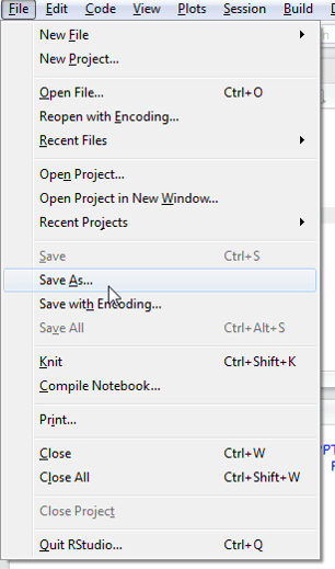
R Source file and Scripts

R script or code file
Can be used to re execute the stored codes
Hit Ctrl+enter to execute the commands
Save R script files for future use.

Saving R Script

Saving & Loading R Work Image

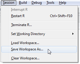
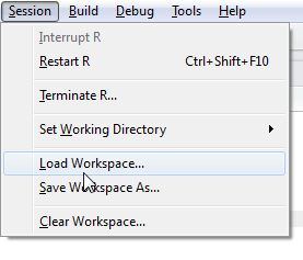
Saves all the R objects, including lists, arrays, data frames Saves all the R objects, including lists, arrays, data frames. Loads the previous working image

Comments

Use # for commenting

#CO2   data is in datasets()
CO2

##    Plant        Type  Treatment conc uptake
## 1    Qn1      Quebec nonchilled   95   16.0
## 2    Qn1      Quebec nonchilled  175   30.4
## 3    Qn1      Quebec nonchilled  250   34.8
## 4    Qn1      Quebec nonchilled  350   37.2
## 5    Qn1      Quebec nonchilled  500   35.3
## 6    Qn1      Quebec nonchilled  675   39.2
## 7    Qn1      Quebec nonchilled 1000   39.7
## 8    Qn2      Quebec nonchilled   95   13.6
## 9    Qn2      Quebec nonchilled  175   27.3
## 10   Qn2      Quebec nonchilled  250   37.1
## 11   Qn2      Quebec nonchilled  350   41.8
## 12   Qn2      Quebec nonchilled  500   40.6
## 13   Qn2      Quebec nonchilled  675   41.4
## 14   Qn2      Quebec nonchilled 1000   44.3
## 15   Qn3      Quebec nonchilled   95   16.2
## 16   Qn3      Quebec nonchilled  175   32.4
## 17   Qn3      Quebec nonchilled  250   40.3
## 18   Qn3      Quebec nonchilled  350   42.1
## 19   Qn3      Quebec nonchilled  500   42.9
## 20   Qn3      Quebec nonchilled  675   43.9
## 21   Qn3      Quebec nonchilled 1000   45.5
## 22   Qc1      Quebec    chilled   95   14.2
## 23   Qc1      Quebec    chilled  175   24.1
## 24   Qc1      Quebec    chilled  250   30.3
## 25   Qc1      Quebec    chilled  350   34.6
## 26   Qc1      Quebec    chilled  500   32.5
## 27   Qc1      Quebec    chilled  675   35.4
## 28   Qc1      Quebec    chilled 1000   38.7
## 29   Qc2      Quebec    chilled   95    9.3
## 30   Qc2      Quebec    chilled  175   27.3
## 31   Qc2      Quebec    chilled  250   35.0
## 32   Qc2      Quebec    chilled  350   38.8
## 33   Qc2      Quebec    chilled  500   38.6
## 34   Qc2      Quebec    chilled  675   37.5
## 35   Qc2      Quebec    chilled 1000   42.4
## 36   Qc3      Quebec    chilled   95   15.1
## 37   Qc3      Quebec    chilled  175   21.0
## 38   Qc3      Quebec    chilled  250   38.1
## 39   Qc3      Quebec    chilled  350   34.0
## 40   Qc3      Quebec    chilled  500   38.9
## 41   Qc3      Quebec    chilled  675   39.6
## 42   Qc3      Quebec    chilled 1000   41.4
## 43   Mn1 Mississippi nonchilled   95   10.6
## 44   Mn1 Mississippi nonchilled  175   19.2
## 45   Mn1 Mississippi nonchilled  250   26.2
## 46   Mn1 Mississippi nonchilled  350   30.0
## 47   Mn1 Mississippi nonchilled  500   30.9
## 48   Mn1 Mississippi nonchilled  675   32.4
## 49   Mn1 Mississippi nonchilled 1000   35.5
## 50   Mn2 Mississippi nonchilled   95   12.0
## 51   Mn2 Mississippi nonchilled  175   22.0
## 52   Mn2 Mississippi nonchilled  250   30.6
## 53   Mn2 Mississippi nonchilled  350   31.8
## 54   Mn2 Mississippi nonchilled  500   32.4
## 55   Mn2 Mississippi nonchilled  675   31.1
## 56   Mn2 Mississippi nonchilled 1000   31.5
## 57   Mn3 Mississippi nonchilled   95   11.3
## 58   Mn3 Mississippi nonchilled  175   19.4
## 59   Mn3 Mississippi nonchilled  250   25.8
## 60   Mn3 Mississippi nonchilled  350   27.9
## 61   Mn3 Mississippi nonchilled  500   28.5
## 62   Mn3 Mississippi nonchilled  675   28.1
## 63   Mn3 Mississippi nonchilled 1000   27.8
## 64   Mc1 Mississippi    chilled   95   10.5
## 65   Mc1 Mississippi    chilled  175   14.9
## 66   Mc1 Mississippi    chilled  250   18.1
## 67   Mc1 Mississippi    chilled  350   18.9
## 68   Mc1 Mississippi    chilled  500   19.5
## 69   Mc1 Mississippi    chilled  675   22.2
## 70   Mc1 Mississippi    chilled 1000   21.9
## 71   Mc2 Mississippi    chilled   95    7.7
## 72   Mc2 Mississippi    chilled  175   11.4
## 73   Mc2 Mississippi    chilled  250   12.3
## 74   Mc2 Mississippi    chilled  350   13.0
## 75   Mc2 Mississippi    chilled  500   12.5
## 76   Mc2 Mississippi    chilled  675   13.7
## 77   Mc2 Mississippi    chilled 1000   14.4
## 78   Mc3 Mississippi    chilled   95   10.6
## 79   Mc3 Mississippi    chilled  175   18.0
## 80   Mc3 Mississippi    chilled  250   17.9
## 81   Mc3 Mississippi    chilled  350   17.9
## 82   Mc3 Mississippi    chilled  500   17.9
## 83   Mc3 Mississippi    chilled  675   18.9
## 84   Mc3 Mississippi    chilled 1000   19.9

CO2$Type

##  [1] Quebec      Quebec      Quebec      Quebec      Quebec     
##  [6] Quebec      Quebec      Quebec      Quebec      Quebec     
## [11] Quebec      Quebec      Quebec      Quebec      Quebec     
## [16] Quebec      Quebec      Quebec      Quebec      Quebec     
## [21] Quebec      Quebec      Quebec      Quebec      Quebec     
## [26] Quebec      Quebec      Quebec      Quebec      Quebec     
## [31] Quebec      Quebec      Quebec      Quebec      Quebec     
## [36] Quebec      Quebec      Quebec      Quebec      Quebec     
## [41] Quebec      Quebec      Mississippi Mississippi Mississippi
## [46] Mississippi Mississippi Mississippi Mississippi Mississippi
## [51] Mississippi Mississippi Mississippi Mississippi Mississippi
## [56] Mississippi Mississippi Mississippi Mississippi Mississippi
## [61] Mississippi Mississippi Mississippi Mississippi Mississippi
## [66] Mississippi Mississippi Mississippi Mississippi Mississippi
## [71] Mississippi Mississippi Mississippi Mississippi Mississippi
## [76] Mississippi Mississippi Mississippi Mississippi Mississippi
## [81] Mississippi Mississippi Mississippi Mississippi
## Levels: Quebec Mississippi

CO2$Type #Printing a column

##  [1] Quebec      Quebec      Quebec      Quebec      Quebec     
##  [6] Quebec      Quebec      Quebec      Quebec      Quebec     
## [11] Quebec      Quebec      Quebec      Quebec      Quebec     
## [16] Quebec      Quebec      Quebec      Quebec      Quebec     
## [21] Quebec      Quebec      Quebec      Quebec      Quebec     
## [26] Quebec      Quebec      Quebec      Quebec      Quebec     
## [31] Quebec      Quebec      Quebec      Quebec      Quebec     
## [36] Quebec      Quebec      Quebec      Quebec      Quebec     
## [41] Quebec      Quebec      Mississippi Mississippi Mississippi
## [46] Mississippi Mississippi Mississippi Mississippi Mississippi
## [51] Mississippi Mississippi Mississippi Mississippi Mississippi
## [56] Mississippi Mississippi Mississippi Mississippi Mississippi
## [61] Mississippi Mississippi Mississippi Mississippi Mississippi
## [66] Mississippi Mississippi Mississippi Mississippi Mississippi
## [71] Mississippi Mississippi Mississippi Mississippi Mississippi
## [76] Mississippi Mississippi Mississippi Mississippi Mississippi
## [81] Mississippi Mississippi Mississippi Mississippi
## Levels: Quebec Mississippi

LAB- My First R program

Create income data(vector) for 4 employees with the values 5500, 6700, 8970, 5634
Create a new variable tax and save 0.2 in it
Create a new variable year and save 2015 in it
Create a new variable company and save “DataVedi” in it
Derive net_income by deducting tax from the income
Create Employee name(vector) for 4 employees with the values Redd, Kenn, Finn, Scott
Create a data frame with Employee name and Net income
Create a new list with all the above information on company, year, tax, Employee name and Salary dataset

Solution

Income<- c(5500, 6700, 8970, 5634)
Tax<-0.2
Year<-2015
Company<-"DataVedi" 
Net_income<- Income*(1-Tax)
Emp_name<-c("Redd", "Kenn", "Finn", "Scott")
Emp_database<-data.frame(Net_income, Emp_name)
Emp_db_list<-list(Income,Tax, Year, Company, Emp_database)

R- Functions

We are already using some functions like c(), is.vector(), str()
Numeric Functions
abs(x), sqrt(x), ceiling(x), floor(x), trunc(x), round(x, digits=n) ,signif(x, digits=n), cos(x), sin(x), tan(x) ,log(x), log10(x), exp(x)
String Functions
substr(x, start=n1, stop=n2), toupper(x), grep(pattern, x , ignore.case=FALSE, fixed=FALSE)

y<-abs(-20)
x<-sum(y+5)
Z<-log(x)
round(Z,1)

## [1] 3.2

cust_id<-"Cust1233416"
id<-substr(cust_id, 5,10)
Up=toupper(cust_id)
grep(4, cust_id)

## [1] 1

Most Common Errors in R

While executing the code on R, its very likely that we get some error.
There are some common errors like syntax & missing packages. By following the below check list you can quickly fix the code errors
Could not find the object: Error: object ‘XXXXX’ not found
Two reasons; The object really not there or most of the times it’s the problem with upper and lower case. We declared as myvar and trying to use it as Myvar
The first check that you should perform is to look the upper and lower case of names

myvar <- c(15, 17, 16, 15, 16)
Myvar
Error: object 'Myvar' not found

Could not find the specific function: Error: could not find function “qplot”
Occurs when the relevant package is missing.
Can fix it by simply installing/attaching the package that contains the function

qplot(mpg, wt, data=mtcars)
Error: could not find function 'qplot'
library(ggplot2)
qplot(mpg, wt, data=mtcars)

Non-numeric argument to binary operator or Invalid ‘type’ (xxxx) of argument
Occurs when we try to apply numeric functions on non numeric variables

Name<- c("John", "Bob", "Kevin", "Smith", "Rick")
Name+1

No such file or directory:
File really doesn’t exists
Most of times file exists, but the path or file name might be wrong or misspelled.
The package is incompatible or built for old version of R.
Need to install the latest version of the package

R-Help

Help home

help.start()

Help on specific functions and usage

?substr()
help(substr)

Conclusion

In this session we covered the basics of R.
We need to be very comfortable with all the topics discussed in this session.
We will be using these topics very often while working on R.
In later sessions we will discuss Data handling techniques.

Handout – Introduction to R

You can download the datasets and R code file for this session here.

R Introduction

Contents

Introduction

What is R

R- A Comprehensive Analytical Tool

Download and Install R

R-Studio

Download and Install R-Studio

Three Main Windows

R Console

R – Quick Warm-up

Workspace

The Assign Operator

Naming convention

LAB: Working with R

R Packages

Download & Install Package

Load a package

LAB: Installing packages

Code: Installing packages

Some Useful Packages in R

R- Data Types

R Vectors

R Vectors

Accessing Vector Elements

Vector Types

R Data frames

Accessing R Data Frames

Difference in Accessed Data frame elements

Built-in Data Frames

Lists

Lists Example

Other Data types

Factors Example

R History

R Source file and Scripts

Saving R Script

Saving & Loading R Work Image

Comments

LAB- My First R program

Solution

R- Functions

Most Common Errors in R

R-Help

Conclusion