You can download the datasets and R code file for this session here.
Introduction
In this chapter we will discuss about logistic regression. Earlier we have talked about the linear regression or it can be also called as regression analysis.Now we will be studying about the logistic regression and how the logistic regression will be different from the linear regression.And we will be discussing about the new concepts that we are going to learn in the logistic regression which are not defined in the linear regression.
Contents
- What is the need of logistic regression?
- Building logistic Regression line
- Goodness of fit measures
- Multicollinearity
- Individual Impact of variables
- Model selection
Regression Recap
In Regression,the dependent variable is predicted using independent variables. A straight line is fit to capture the relation in the form of a model. The R-Square/ Adjusted R-Square values tell us the goodness of fit of the model. Once the line is ready we can substitute the values of x(predictor) to get the predicted values of y(dependent variable).
LAB: Regression – Recap
- Import Dataset: Product Sales Data/Product_sales.csv
- What are the variables in the dataset?
- Build a predictive model for Bought vs Age
- What is R-Square?
- If Age is 4 then will that customer buy the product?
- If Age is 105 then will that customer buy the product?
- Draw a scatter plot between Age and Buy. Include the regression line on the same chart.
Solution
- Import Dataset: Product Sales Data/Product_sales.csv
Product_sales <- read.csv("~R datasetProduct Sales DataProduct_sales.csv")Here is the Product Sales Dataset, where we are having two variables which can be predicted. The "Bought" vs. "Age" will be the two variables that can have different values. "Bought" will be having two values, i.e., "Yes" or "No". While "Age" will be based on the customer's age. We have to just predict whether the customer will buy the product or not according to their age. Thus for that we have to create linear regression between "Bought" and "Age". Then we have to find the R-Square. We have to find if the customer's age is 4, then that customer will buy the product or not. And if the customer's age is 105, then the customer will buy the product or not.
- What are the variables in the dataset?
names(Product_sales)## [1] "Age" "Bought"- Build a predictive model for Bought vs Age
prod_sales_model<-lm(Bought~Age,data=Product_sales)
summary(prod_sales_model)
##
## Call:
## lm(formula = Bought ~ Age, data = Product_sales)
##
## Residuals:
## Min 1Q Median 3Q Max
## -1.14894 -0.12800 -0.01807 0.10759 1.10759
##
## Coefficients:
## Estimate Std. Error t value Pr(>|t|)
## (Intercept) -0.1704125 0.0152752 -11.16 <2e-16 ***
## Age 0.0209421 0.0004205 49.80 <2e-16 ***
## ---
## Signif. codes: 0 '***' 0.001 '**' 0.01 '*' 0.05 '.' 0.1 ' ' 1
##
## Residual standard error: 0.1976 on 465 degrees of freedom
## Multiple R-squared: 0.8421, Adjusted R-squared: 0.8418
## F-statistic: 2480 on 1 and 465 DF, p-value: < 2.2e-16- What is R-Square? 0.8421
- If Age is 4 then will that customer buy the product?
new_data<-data.frame(Age=4)
predict(prod_sales_model,new_data)
## 1
## -0.08664394- If Age is 105 then will that customer buy the product?
new_data<-data.frame(Age=105)
predict(prod_sales_model,new_data)
## 1
## 2.028511As you can see here the value comes as 2.028, then this doesn’t mean that the customer is going to buy 2 types of product.There is something wrong with this graph.
- Draw a scatter plot between Age and Buy. Include the regression line on the same chart.
plot(Product_sales$Age,Product_sales$Bought,col = "blue")
abline(prod_sales_model, lwd = 5, col="red")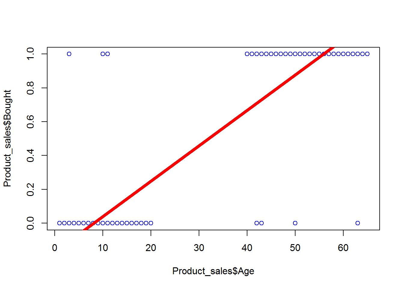
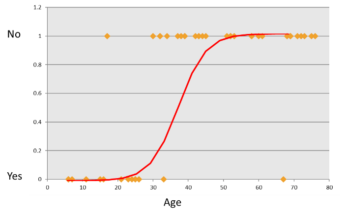
Now as we can see in the graph, this is the incorrect regression line.If you draw the dataset, it is having two variables “Buying” and “Age”.As the “Bought” variable will be having only two answers, i.e., 0 or 1. So we cannot create the linear regression line in this case. Because as we can see, the customer of age 4 won’t be buying the product and the customer of age from particular range i.e., beyond 20 will be buying that product. As you can see it in the graph below, all the 0 values are between 0 to 20 age, while all the 1 values will be beyond 40 age. Thus we cannot draw the linear regression line as it won’t be fit for this data. As we can see in the above figure, we can say that we cannot fit this regression model for the non-linear data. Here the “Buy” variable will be having only two values, 0 and 1. So for this non-linear data, we cannot forcefully fit the linear regression model. And fitting linear regression line for such type of data is wrong. Just for the comparison; in linear regression model, as X variable increases then Y also increases accordingly. We can only fit linear regression line when X and Y both are linear. And here the data is not linear.
What is the need of logistic regression?
Consider Product sales data. The dataset has two columns. + Age – continuous variable between 6-80 + Buy(0- Yes ; 1-No)
plot(Product_sales$Age,Product_sales$Bought,col = "blue")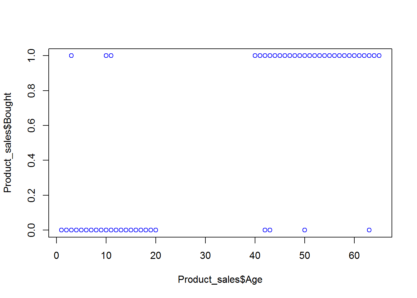
Here we can say that in the above graph we cannot forcefully fit the linear regression line and the model that we built is not right.There is certain issues with the type of dependent variables like the variable “Buy” will be binary. And hence we cannot fit the linear regression line to this data. Now here the question arises that: “Why not linear?”
Real-life examples
Some real life examples for binary functions can be:
- Gaming – Win vs. Loss
- Sales – Buying vs. Not buying
- Marketing – Response vs. No Response
- Credit card & Loans – Default vs. Non Default
- Operations – Attrition vs. Retention
- Websites – Click vs. No click
- Fraud identification – Fraud vs. Non Fraud
- Healthcare – Cure vs. No Cure
Why not linear?
“Age” is the continuous data and it takes values according to the range given (8 to 60). But as we can see the variable “Buy” is not the continuous data. It is binary and has only 0 or 1 data. Hence in the end no matter what we do or no matter what optimization we use, we are not able to fit the linear regression line to this data. Let’s talk about the real life examples.
Some Nonlinear Functions
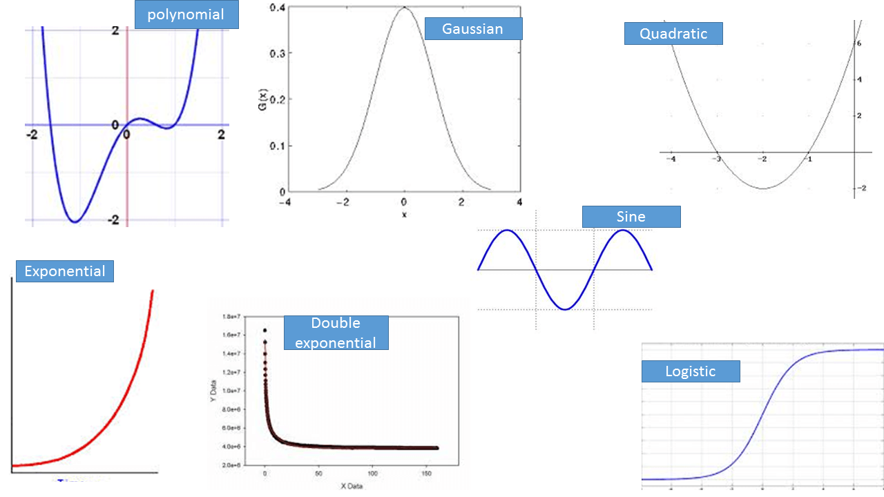
As we can see in the functions given. There is a polynomial function; will that be able to fit for our data? I don’t think so, this will not fit our data. There is a Gaussian function; again this will not fit for our data. There is a quadratic equation; again this will not fit for our data. There is an exponential; again this will not fit for our data. There is a double exponential; again this will not fit our data. There is sine function; again this will not fit for our data. There is logistic function; which we can fit to our data
A Logistic Function
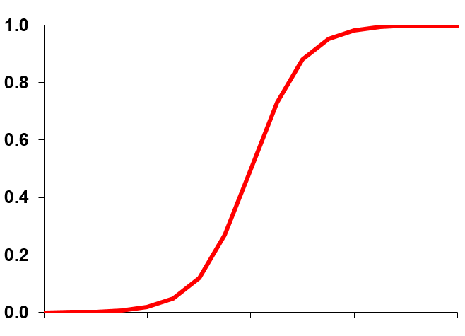
This is the logistic function; which we can fit to our data. This function is S shaped.
The Logistic Function
Even it looks like “S” may be if we adjust some parameters then we can fit the data because it looks like it’s tails are longer and the mid portion is shorter and it will be a good fit to our data set. We will use logistic function to fit to our data rather than linear function. We can even avoid many errors, rather than just fitting the straight line. Earlier the equation of linear regression was . Now for logistic regression we have some what different equation. So for that we need the model that predicts the probabilities between 0 and 1. The model should be in “S” shaped. There is portion of the data, full of 0’s and there is portion of the data, full of 1’s. Some people of age less than 0’s portion are not buying and some people of age more than 1’s are buying. Most of them are the pattern we are observing in the variable. As the variable increases then the other variable is dominating m. Like “Age” is increasing then the “Buying” will be dominating. Now what is the logistic regression equation? Earlier in the linear regression line, the value of equation will be simple equation but for the logistic regression line equation we have this,
The function on left, , is called the logistic function.
Logistic Regression Function
Logistic regression models the logit of the outcome, instead of the outcome i.e. instead of winning or losing, we build a model for log odds of winning or losing. Natural logarithm of the odds of the outcome ln(Probability of the outcome (p)/Probability of not having the outcome (1-p))
Lab: Logistic Regression
- Import Dataset: Product Sales Data/Product_sales.csv
- Build a logistic Regression line between Age and buying
- A 25 years old customer, will he buy the product?
- If Age is 105 then will that customer buy the product?
- Draw a scatter plot between Age and Buy. Include both linear and logistic regression lines on the same chart.
Solution: Logistic Regression in R
- Import Dataset: Product Sales Data/Product_sales.csv
Product_sales<- read.csv("~R datasetProduct Sales DataProduct_sales.csv")- Build a logistic Regression line between Age and buying
prod_sales_Logit_model <- glm(Bought ~ Age,family=binomial(logit),data=Product_sales)
summary(prod_sales_Logit_model)
##
## Call:
## glm(formula = Bought ~ Age, family = binomial(logit), data = Product_sales)
##
## Deviance Residuals:
## Min 1Q Median 3Q Max
## -3.6922 -0.1645 -0.0619 0.1246 3.5378
##
## Coefficients:
## Estimate Std. Error z value Pr(>|z|)
## (Intercept) -6.90975 0.72755 -9.497 <2e-16 ***
## Age 0.21786 0.02091 10.418 <2e-16 ***
## ---
## Signif. codes: 0 '***' 0.001 '**' 0.01 '*' 0.05 '.' 0.1 ' ' 1
##
## (Dispersion parameter for binomial family taken to be 1)
##
## Null deviance: 640.425 on 466 degrees of freedom
## Residual deviance: 95.015 on 465 degrees of freedom
## AIC: 99.015
##
## Number of Fisher Scoring iterations: 7- A 25 years old customer, will he buy the product?
new_data<-data.frame(Age=25)
predict(prod_sales_Logit_model,new_data,type="response")
## 1
## 0.1879529- If Age is 105 then will that customer buy the product?
new_data<-data.frame(Age=105)
predict(prod_sales_Logit_model,new_data,type="response")
## 1
## 0.9999999- Draw a scatter plot between Age and Buy. Include both linear and logistic regression lines on the same chart.
plot(Product_sales$Age,Product_sales$Bought,col = "blue")
curve(predict(prod_sales_Logit_model,data.frame(Age=x),type="resp"),add=TRUE)
abline(prod_sales_model, lwd = 5, col="red")
Multiple Logistic Regression We discussed about the single logistic regression. Why it is simple logistic regression? Because there we take only one single predictor variable to predict the output variable i.e., we used only “Age” predictor to use “Buy”. But in real life we won’t be having the scenario where only one variable will be impacting the target variable. There can be multiple variables that can be impacting the target variables. Now here the output variable is binary. Instead of single independent/predictor variable, we have multiple predictor variables then we have to build multiple logistic regression line instead of single logistic regression line. The idea is very much similar to the multiple linear regression line that we have built. We have created multiple linear regression line instead of single linear regression line because there are various factors that are impacting on the target variable. In the same way, the customer’s attributes like age, gender, income, place, buying patterns, expense, etc. are all depend on the buying/ non buying of the product. The model will be the same as in the logistic regression i.e., the predictor list will be multiple compared to the single logistic regression where only one predictor was there. We just have to build the multiple logistic regression line by taking the multiple predictor inputs. Everything else is similar just as the single logistic regression like the output will be again the buying/non buying and the output will be again the same binary values i.e., 0 or 1. The line will be the multi-dimensional. Now building the multiple logistic regression line.
LAB: Multiple Logistic Regression
There is a dataset called Fiberbits data and this is an internet service provider dataset. Since last few years, there were some customers who stick with this service provider and there were also some customers who left this service provider. Now what we are trying to do is to build an attrition kind of model that will check whether the customer will be there or not. We are trying to do these things because if we get to know who are going to leave and who are going to stick to this service provider then we can send them promotional code and offers to retain to this service provider. So Active_cust is the variable from which we can able to retrieve whether the customer is active or already left the network. There might be other variables that will be used as predictor variables. There are many reasons for the customers to stay back or leave the network. We will try to build the model that will predict whether the customer will stay back or the customer will leave. And the model that we have to build is on the fiberbits data.
-
- Import Dataset: Fiberbits/Fiberbits.csv
- Active_cust variable indicates whether the customer is active or already left the network.
-
- Build a model to predict the chance of attrition for a given customer using all the features.
-
- How good is your model?
Solutions
- Import Dataset: Fiberbits/Fiberbits.csv
Fiberbits <- read.csv("~R datasetFiberbitsFiberbits.csv")Here, the fiberbits data is having 100000 rows and 9 columns. Columns like active_cust which is having the value 0 or 1 and is the target variable, i.e., being in the network and leaving the network depends on the income, months on network, number of complaints they gave, number of plan changes they made, relocation status is like whether they relocated or not, the monthly bill that they are getting, technical issues per month and speed test results like whatever the speed they promised whether they gave it or not. Every criterion is there in this dataset. The task is we have to predict whether the customer is going to stick to this service provider or that customer is going to leave the network depending on all the criteria that we have mentioned. Now here the active customer is having the values 0 or 1, hence directly we are going to build the model using rest of the variables. Here, the model will be depending on the active customer versus all the other variables. If we are defining all the variables then we can write like,
- Build a model to predict the chance of attrition for a given customer using all the features.
Fiberbits_model_1<-glm(active_cust~.,family=binomial(),data=Fiberbits)## Warning: glm.fit: fitted probabilities numerically 0 or 1 occurredsummary(Fiberbits_model_1)##
## Call:
## glm(formula = active_cust ~ ., family = binomial(), data = Fiberbits)
##
## Deviance Residuals:
## Min 1Q Median 3Q Max
## -8.4904 -0.8752 0.4055 0.7619 2.9465
##
## Coefficients:
## Estimate Std. Error z value Pr(>|z|)
## (Intercept) -1.761e+01 3.008e-01 -58.54 <2e-16 ***
## income 1.710e-03 8.213e-05 20.82 <2e-16 ***
## months_on_network 2.880e-02 1.005e-03 28.65 <2e-16 ***
## Num_complaints -6.865e-01 3.010e-02 -22.81 <2e-16 ***
## number_plan_changes -1.896e-01 7.603e-03 -24.94 <2e-16 ***
## relocated -3.163e+00 3.957e-02 -79.93 <2e-16 ***
## monthly_bill -2.198e-03 1.571e-04 -13.99 <2e-16 ***
## technical_issues_per_month -3.904e-01 7.152e-03 -54.58 <2e-16 ***
## Speed_test_result 2.222e-01 2.378e-03 93.44 <2e-16 ***
## ---
## Signif. codes: 0 '***' 0.001 '**' 0.01 '*' 0.05 '.' 0.1 ' ' 1
##
## (Dispersion parameter for binomial family taken to be 1)
##
## Null deviance: 136149 on 99999 degrees of freedom
## Residual deviance: 98359 on 99991 degrees of freedom
## AIC: 98377
##
## Number of Fisher Scoring iterations: 8Here the model building is been done. This is the model which helps us to predict but the equation is somewhat complicated here. Looking at the coefficients values of all the variables, we can say if the value of probability by substituting all the variables is 1 or near to 1, then the customer might leave the network and if the probability is 0 or near to 0, then the customer will not leave the network. If the probability is near to 1, then we can start building the strategies or we can start segmenting out the customer thus to somehow retain them. Its not only about the internet service provider but we can use this model in any field which gives the binary values. Thus we can build the multiple logistic regression line.
Goodness of Fit for a Logistic Regression
After building the logistic regression line, the question arises that how good the model is? If someone challenges that the line which is been fitted in the model is not right or what is the confidence in your prediction or how good is your model or what is the goodness of fit of the particular model. What is the goodness of the fit measures in a logistic regression? If you observe carefully, then R2 is not a right measure because in percentage of variation explained by all the predictor variables in Y. Thus the Y’s variance is how much percentage of variance is explained or how much percentage is predicted by all the variables. Here the Y variables are taking two values and there will be hardly any variance i.e., 1 or 0. Hence R2 is not the right measure of goodness of fit for logistic regression. There are other ways of finding out the way of goodness of fit for logistic regression as follows: – Classification Matrix – AIC and BIC = ROC and AUC – Area under the curve
Classification Table & Accuracy
Now discussing about the confusion matrix which is also called the classification model which gives the accuracy of the model. If we understand that Y takes two values in the action then it will be like Yes or No, 1 or 0, (-1) or (+1), True or False, etc. and at the end of the prediction in our model, we are also going to give two values 0 or 1, Yes or No, etc. Take a data point that already exists in the data. Suppose let’s take a point active_cust is 0 and then observe all the variables that are given for that data and build the model. With that logistic regression model, if we substitute every other variables and the prediction comes to be 0 or near to 0, then we are doing good because the actual value is 0. But we substitute every other value and the prediction comes to be 1 then at that particular point you have made a mistake and that is the wrong prediction. Hence we want to have some lesser such wrong predictions. For the good model, when the actual value is 0 and you want to predict as 0 by substituting all the variables, thus 0 should be predicted as 0 and 1 should be predict as 1. If 0 is predicted as 1 and 1 is predicted as 0 then that is wrong prediction or misclassification. The predicted values are not 0 and 1, they are probabilities. And the probabilities will be in between 0 and 1. We can put the threshold like, anything more than 0.5 will be 1 and anything less than 0.5 will be 0. Hence the actual value is 0 and we are getting the probability value which is near to 0 then our model is right. Let’s suppose there are dataset in which there are 1000 data points. Out of which 500 zero’s are there and 500 one’s are there. Hence most of the 500 zero’s should be predicted as 0’s. But may be some values are predicted as 1. Most of the 1 should be predicted as 1, and then only we can say that the model is a good one.
| Predicted / Actual | 0 | 1 |
|---|---|---|
| 0 | True Positive (TP) | False Positive (FP) |
| 1 | False Negative (FN) | True Negative (TN) |
As seen in the table, if the “True Positives” and “True Negatives” will be lesser and “False Positives” and “False Negatives” will be higher then there will be something wrong in the prediction. (Here the True Positives, True Negatives, etc. will be further discussed.) For a good model, all 0 should be predicted as 0 and all 1 should be predicted as 1. The given table is called the confusion matrix or classification table. Accuracy is predicting the 0 as 0 and 1 as 1 i.e., these diagonals elements is the accuracy. (Right now just consider them as the diagonals elements.) Accuracy is what percentage of time and how many times out of overall cases you are predicting them correctly. Hence for your model you need to find out accuracy. Accuracy is been always derived only by classification table or confusion matrix. In fact, 0 is considered as positive and 1 is considered as negative.The rows are the actual classes and the columns are the predicted classes. When 0 is predicted as 0, then they are called True Positive which is like when actual condition is Positive, it is truly predicted as positive. When 0 is predicted as 1, then they are called False Negative which is like when actual condition is Positive, it is falsely predicted as negative. When 1 is predicted as 0, then they are called False Positives which is like when actual condition is Negative, it is falsely predicted as positive. When 1 is predicted as 1, then they are called True Negatives which is like when actual condition is Negative, it is truly predicted as negative. Hence there should be high number of “True Positives” and “True Negatives”, and there should be less number of “False Positives” and “False Negatives”.
Misclassification= 1- Accuracy We can also derived Specificity and Sensitivity from confusion matrix. As of now we are concentrating in the accuracy for the logistic regression line. By observing the accuracy and confusion matrix, we can decide whether the model is good or bad. Any accuracy with more than 80% is really good. Most of the time it depends on the data, if the data is really good then it gives higher accuracy and vice versa.
Classification Table in R
threshold=0.5
predicted_values<-ifelse(predict(prod_sales_Logit_model,type="response")>threshold,1,0)
actual_values<-prod_sales_Logit_model$y

conf_matrix<-table(predicted_values,actual_values)
conf_matrix
##                    actual_values
## predicted_values      0    1
##                0     257   3
##                1      5   202
Accuracy in R
accuracy<-(conf_matrix[1,1]+conf_matrix[2,2])/(sum(conf_matrix))
accuracy
## [1] 0.9828694Multicollinearity
Multicollinearity is nothing but the interdependency of the predictor variables. Within predictor variables some variables are interdependent. At the time of interdependence, the final regression coefficients went for a toss, the variance of coefficients was very high that we cannot trust the coefficients. When we are doing the individual impact of analysis say X1, X2 or related and when we are doing the relation analysis as X1 versus Y and X2 versus Y because, the coefficients are wrong and we are getting into wrong conclusions. Then we realize that X1 and X2 are related and that is called multicollinearity. We just cannot keep both of them in the model at the same time; it has to be X1 or X2 because one of them is carrying the complete information about the other one. By observing we get to know that multicollinearity is only related to predictor variables, it has nothing to do with Y versus X. It totally depends on X versus remaining all X’s, X1 versus remaining all X’s or X2 versus remaining all X’s. Now multicollinearity is an issue even in logistic regression because we are hardly considering the Y or dependent variable in that scenario. Thus if there is multicollinearity then the logistic regression coefficients will go for a toss. Multicollinearity needs to be treated in the logistic regression because even in logistic regression we are using some kind of optimization when there are variables which are interlinked within this model. Definitely they are going to impact the coefficients and again they are going to led to wrong conclusion even in logistic regression when we are trying to analyse the impact of the each variable i.e., the Y variable. So multicollinearity needs to be treated even in logistic regression. The relation between X and Y is non-linear, that is why we are using logistic regression. The multicollinearity is an issue related to predictor variables. Multicollinearity needs to be fixed even in logistic regression as well. Otherwise the individual coefficients will be affected. The process of identification of multicollinearity is same as the logistic regression because multicollinearity is all about the relation within X variables i.e., X1 versus remaining variables that is how we find the VIF (Variance inflation factors) values. We just have to find VIF values which is derived from indeed when we build individual model i.e., X versus remaining variables. Hence we have to use VIF values to identify multicollinearity. If it is multicollinearity then we can give same treatment that we were giving it earlier.
Multicollinearity in R
We take the “Fiberbits” Dataset and for multicollinearity we need to find VIF. Any VIF value more than 5, which is an indication of multicollinearity. But that doesn’t mean we have to drop all the variables that the VIF value are having more than 5. We will drop one by one variable. Hence X1 is depending on X2 and X2 is depending on X1, then X2 is redundant in presence of X1 and X1 is redundant in presence of X2. So both of them will have VIF more than 5, but that does not mean we should drop both X1 and X2, we will lose out the basic information. For multicollinearity we need to drop out one by one only. First find out the VIF, go for the highest VIF, then observe is there any VIF that is more than 5 then we can drop the highest variable of VIF.
library(car)
vif(Fiberbits_model_1)
## income months_on_network
## 4.590705 4.641040
## Num_complaints number_plan_changes
## 1.018607 1.126892
## relocated monthly_bill
## 1.145847 1.017565
## technical_issues_per_month Speed_test_result
## 1.020648 1.206999We need to use car package which is companion to use applied regression and then summary of the model and then we have to use VIF function. As we can see no variable is having more than 5 VIF value, then it means that all the variables will be having independent information. We cannot drop the variables that are nearer values to 5, because if we drop it then we may lose out on some information that might impact the overall accuracy of our model. Hence that is how we find out multicollinearity. Multicollinearity is only applicable when the model has multiple independent variables. It is to test whether there are any variables carrying same information but named as two different variables. Multicollinearity is depends on the questions like why we need to eliminate multicollinearity and how multicollinearity is also known as redundancy.
Individual Impact of Variables
Out of all the predictor variables that we have used for prediction of the buying or non-buying or that we have used for attrition versus non-attrition, hence the question arises is what are the important variables? If we have to choose top 5 variables then what will be those variables? While selecting any model, is there any way that we can drop the variables that are not impacting or that are less impacting and keep only the important variables thus we don’t have to collect or maintain the data for those less impacting variables. Why should we keep the variables those who are not impacting? How to rank the predictor variables in order of their importance? Individual Impact – z-values and Wald Chi-square How do we find out the individual impact of the variables? The answer is for finding out the individual impact of the variables; we have to observe the z-values and Wald-chi square. There are z-values in our output against each variable. Observing the z-values or the absolute values of the z, we can say the impact of that variable. We can rank them by observing the Wald Chi-square or the square of the z-values. We have to simply square that z-value, that the variable with highest z-value will be the best one. Talking about absolute value, if you have the variable with z-value as (-30) and another variable with z-value as 10, the most important variable will be the variable with z-value as (-30) because some variables might be positively impacting while some variables might be negatively impacting but it only depends on impact thus we have to consider as absolute z-value. Or in simple terms we have to consider the Wald Chi square value or Chi-square value or the z-square value. Let’s observe what are the top impacting variable or how do we rank the variable in our fiberbits data.
Code-Individual Impact of Variables
Identify the top impacting and least impacting variables in fiberbits data. Find the variable importance and order them based on their impact.
library(caret)## Loading required package: lattice## Loading required package: ggplot2varImp(Fiberbits_model_1, scale = FALSE)## Overall
## income 20.81981
## months_on_network 28.65421
## Num_complaints 22.81102
## number_plan_changes 24.93955
## relocated 79.92677
## monthly_bill 13.99490
## technical_issues_per_month 54.58123
## Speed_test_result 93.43471This will give the absolute value of the Z-score
Model Selection – AIC and BIC
While trying to build the best model, we tend to add many variables, we tend to derive many variables, we tend to add many data and we sometimes try to build an optimal model by dropping the variables. For improving the model, there are many possibilities which we can implement it.
- By adding new independent variables
- By deriving new variables
- By transforming variables
- By collecting more data
Or sometimes we want to just to drop the few variables even if we have to reduce or even if we lose out some of the accuracy. May be instead of building a model with 200 or 300 variables, we want to build a model with just 50 or 60 variables or may be 20 variables and have the best accuracy possible. We can have the most top impacting variable and have an accuracy of 80%, rather than having 200-300 variables and accuracy of 85%.Thus how do we build if we have several models with same accuracy level or how do we choose best models or how do we choose the model that is best suited or how do we choose the optimal model for a given set of parameters for given accuracy level. Considering that there are different models called M1, M2 or M3 then how do we get to know that M1 or M2 or M3 is apt model for the data? Hence that question can be answered by observing the AIC (Akaike Information Criterion) and BIC (Bayesian Information Criterion) values. AIC and BIC values of given model or standalone AIC has no real use and has something like Adjusted R-square in linear regression. When we have 2-3 models; by observing the AIC values, the best fit is the model with least AIC values. AIC is an estimate of information that is loss when a given model is use to represent the process that generates the data or simply AIC is the information loss while building the model. Hence we want to lose the least amount of information while building the model. If you have two models; model-1 and model-2, then compare accuracy between them. Let’s say the model-1 is having accuracy of 84% and model-2 is having accuracy of 85% and we want to choose a model, because model-1 is built on 20 variables and model-2 is built on 30 variables and we want to know that on which model we want to go with. Then based on AIC, we have to choose the model that has least information loss which is best model. AIC formula includes the maximum likelihood function for the model and number of parameters as well. AIC= -2ln(L)+ 2k
- L be the maximum value of the likelihood function for the model
- k is the number of independent variables
Hence if we have multiple numbers of parameters or if we are having too many independent variables, then we can observe the AIC value. For a given accuracy, if we want to choose the best model then we have to observe the AIC value. AIC is information loss. If we have the 2-3 models of same level of accuracy i.e., all the models called M1, M2, M3, etc. have same nearby accuracy values, then we can know the best model out of them. For finding the best model out of all of the others and the least information loss model is been calculated by AIC. Now discussing about BIC; BIC is just a substitute to AIC which is having slightly different formula. We can either AIC or BIC (one of them is sufficient or we can simply fixed to AIC) throughout our analysis.
Code-AIC and BIC
library(stats)
AIC(Fiberbits_model_1)
## [1] 98377.36BIC(Fiberbits_model_1)## [1] 98462.97LAB-Logistic Regression Model Selection
- What are the top-2 impacting variables in fiber bits model?
- What are the least impacting variables in fiber bits model?
- Can we drop any of these variables?
- Can we derive any new variables to increase the accuracy of the model?
- What is the final model? What the best accuracy that you can expect on this data?
Solution
- What are the top-2 impacting variables in fiber bits model?
Speed_test_result and relocation status are the top two important variables
- What are the least impacting variables in fiber bits model?
monthly_bill and income are the least impacting variables
- Can we drop any of these variables?
We can drop monthly_bill and income, they have the least impact when compared to other predictors. But we need to see the accuracy and AIC then take the final decision.
AIC & Accuracy of Model1
threshold=0.5

predicted_values<-ifelse(predict(Fiberbits_model_1,type="response")>threshold,1,0)
actual_values<-Fiberbits_model_1$y

conf_matrix<-table(predicted_values,actual_values)
conf_matrix
## actual_values
## predicted_values 0 1
## 0 29492 10847
## 1 12649 47012accuracy1<-(conf_matrix[1,1]+conf_matrix[2,2])/(sum(conf_matrix))
accuracy1## [1] 0.76504AIC(Fiberbits_model_1)## [1] 98377.36As we are finding the accuracy of model-1 and the accuracy of model-1 will be 76% that we have already found at fiberbits data. Accuracy is 76% with the threshold of 0.5.
AIC & Accuracy of Model1 without monthly_bill
Fiberbits_model_11<-glm(active_cust~.-monthly_bill,family=binomial(),data=Fiberbits)## Warning: glm.fit: fitted probabilities numerically 0 or 1 occurredthreshold=0.5
predicted_values<-ifelse(predict(Fiberbits_model_11,type="response")>threshold,1,0)
actual_values<-Fiberbits_model_11$y
conf_matrix<-table(predicted_values,actual_values)
accuracy11<-(conf_matrix[1,1]+conf_matrix[2,2])/(sum(conf_matrix))
accuracy11## [1] 0.76337AIC(Fiberbits_model_11)## [1] 98580.54Here the variable called income is one of the least impacting variables after monthly_bill thus we will try to drop income and build the model-2.AIC & Accuracy of Model1 without income
Fiberbits_model_2<-glm(active_cust~.-income,family=binomial(),data=Fiberbits)## Warning: glm.fit: fitted probabilities numerically 0 or 1 occurredthreshold=0.5
predicted_values<-ifelse(predict(Fiberbits_model_2,type="response")>threshold,1,0)
actual_values<-Fiberbits_model_2$y
conf_matrix<-table(predicted_values,actual_values)
accuracy2<-(conf_matrix[1,1]+conf_matrix[2,2])/(sum(conf_matrix))
accuracy2## [1] 0.76695AIC(Fiberbits_model_2)## [1] 99076.27Here, we can see that the information loss in model-1 is 98377.36 and that in model-2 is 99076.27. If we drop one more variable then the information loss will be higher. We have to observe that are we able to cop up with dropping of one variable. We will be rather gone for model-2 because the information loss is higher but it is not that much important loss of information as the accuracy is almost same and we don’t need to maintain that variable. But if by dropping that variable we are losing a lot of information then we will not choose that model.
Deciding which Variable to Drop
| Model | All Variables | Without monthly_bill | Without income |
|---|---|---|---|
| AIC | 98377.36 | 98580.54 | 99076.27 |
| Accuracy | 0.76504 | 0.76337 | 0.76695 |
Dropping Income has not reduced the accuracy. AIC(Loss of information) also shows no big change.
Output of Model2
summary(Fiberbits_model_2)##
## Call:
## glm(formula = active_cust ~ . - income, family = binomial(),
## data = Fiberbits)
##
## Deviance Residuals:
## Min 1Q Median 3Q Max
## -8.4904 -0.8901 0.4175 0.7675 3.1083
##
## Coefficients:
## Estimate Std. Error z value Pr(>|z|)
## (Intercept) -1.309e+01 2.100e-01 -62.34 <2e-16 ***
## months_on_network 1.004e-02 4.644e-04 21.62 <2e-16 ***
## Num_complaints -7.071e-01 2.990e-02 -23.65 <2e-16 ***
## number_plan_changes -2.016e-01 7.571e-03 -26.63 <2e-16 ***
## relocated -3.133e+00 3.933e-02 -79.66 <2e-16 ***
## monthly_bill -2.253e-03 1.566e-04 -14.39 <2e-16 ***
## technical_issues_per_month -3.970e-01 7.159e-03 -55.45 <2e-16 ***
## Speed_test_result 2.198e-01 2.334e-03 94.16 <2e-16 ***
## ---
## Signif. codes: 0 '***' 0.001 '**' 0.01 '*' 0.05 '.' 0.1 ' ' 1
##
## (Dispersion parameter for binomial family taken to be 1)
##
## Null deviance: 136149 on 99999 degrees of freedom
## Residual deviance: 99060 on 99992 degrees of freedom
## AIC: 99076
##
## Number of Fisher Scoring iterations: 7- Can we derive any new variables to increase the accuracy of the model?
Fiberbits_model_3<-glm(active_cust~    income
                      +months_on_network
                      +Num_complaints
                      +number_plan_changes
                      +relocated
                      +monthly_bill
                      +technical_issues_per_month
                      +technical_issues_per_month*number_plan_changes
                      +Speed_test_result+I(Speed_test_result^2),
                      family=binomial(),data=Fiberbits)
## Warning: glm.fit: fitted probabilities numerically 0 or 1 occurredsummary(Fiberbits_model_3)##
## Call:
## glm(formula = active_cust ~ income + months_on_network + Num_complaints +
## number_plan_changes + relocated + monthly_bill + technical_issues_per_month +
## technical_issues_per_month * number_plan_changes + Speed_test_result +
## I(Speed_test_result^2), family = binomial(), data = Fiberbits)
##
## Deviance Residuals:
## Min 1Q Median 3Q Max
## -4.6112 -0.8478 0.3780 0.7401 2.9909
##
## Coefficients:
## Estimate Std. Error
## (Intercept) -2.501e+01 3.647e-01
## income 1.831e-03 8.386e-05
## months_on_network 2.905e-02 1.011e-03
## Num_complaints -6.972e-01 3.030e-02
## number_plan_changes -4.404e-01 2.199e-02
## relocated -3.253e+00 3.997e-02
## monthly_bill -2.295e-03 1.588e-04
## technical_issues_per_month -4.670e-01 9.694e-03
## Speed_test_result 3.910e-01 4.260e-03
## I(Speed_test_result^2) -9.438e-04 1.272e-05
## number_plan_changes:technical_issues_per_month 7.481e-02 6.164e-03
## z value Pr(>|z|)
## (Intercept) -68.56 <2e-16 ***
## income 21.83 <2e-16 ***
## months_on_network 28.73 <2e-16 ***
## Num_complaints -23.00 <2e-16 ***
## number_plan_changes -20.03 <2e-16 ***
## relocated -81.39 <2e-16 ***
## monthly_bill -14.46 <2e-16 ***
## technical_issues_per_month -48.17 <2e-16 ***
## Speed_test_result 91.79 <2e-16 ***
## I(Speed_test_result^2) -74.20 <2e-16 ***
## number_plan_changes:technical_issues_per_month 12.14 <2e-16 ***
## ---
## Signif. codes: 0 '***' 0.001 '**' 0.01 '*' 0.05 '.' 0.1 ' ' 1
##
## (Dispersion parameter for binomial family taken to be 1)
##
## Null deviance: 136149 on 99999 degrees of freedom
## Residual deviance: 97105 on 99989 degrees of freedom
## AIC: 97127
##
## Number of Fisher Scoring iterations: 7AIC & Accuracy of Model 3
threshold=0.5

predicted_values<-ifelse(predict(Fiberbits_model_3,type="response")>threshold,1,0)
actual_values<-Fiberbits_model_3$y

conf_matrix<-table(predicted_values,actual_values)
accuracy3<-(conf_matrix[1,1]+conf_matrix[2,2])/(sum(conf_matrix))
accuracy3
## [1] 0.76061AIC(Fiberbits_model_3)## [1] 97127.17- What is the final model? What the best accuracy that you can expect on this data?
AIC(Fiberbits_model_1,Fiberbits_model_2,Fiberbits_model_3)## df AIC
## Fiberbits_model_1 9 98377.36
## Fiberbits_model_2 8 99076.27
## Fiberbits_model_3 11 97127.17accuracy1## [1] 0.76504accuracy2## [1] 0.76695accuracy3## [1] 0.76061As all the models will be having same AIC values and there will be almost same kind of information loss, then it depends on us that what model we want to select. It can be done by depending on the type of the problem, depending on the class of the problem and for specific business problem we are using AIC. Sometimes we want to choose model-3 because it is having least information loss and it has captured everything but the only thing is that it is more complicated than other models. May be we can stick to the model-1, where we can use all the variables and the information loss will not be that much high. Or we can use the model-2, where the information loss is just slightly higher than the model-1 as only one variable is dropped. Hence that is how we can use the AIC and BIC values. If more than one models are doing the same type of work then we can observe the AIC and accuracy and trade-off between them for the best fitted model. Even the BIC is also consistent as compared with AIC, because they never contradict each other and they will be almost same in every manner.
Conclusion:
Here in this chapter, we learnt about the logistic regression, what will be the need of logistic regression, why we need logistic regression when we already have the linear regression, what is the difference between logistic regression and linear regression, how to fit a logistic regression and how to validate the logistic regression, how to do the model selection, etc. Thus the logistic regression is the good foundation of all the algorithms. Hence, if we have good understanding of the logistic regression and goodness of fit measures of logistic regression, then it will really help in understanding complex machine learning algorithms like neural networks and SVMs. Further topics will be much easier compared to this topic. In fact the neural networks is been derived from logistic regression. Hence we have to be very careful while selecting the model and all the goodness of fit measures are calculated on the training data. We may have to do some out of time validation or cross validation to get an idea on actual error or the actual accuracy of the model. So in future topics we will be discussing about the neural networks, SVMs, etc.