You can download the datasets and R code file for this session here.

Introduction

Decision tree is a type of supervised learning algorithm that is mostly used in classification problems.In this technique, we split the population or sample into two or more homogeneous sets based on most significant differentiator in input variables.

What is segmentation
Segmentation Business Problem
Decision Tree Approach
Splitting Criterion
Impurity or Diversity Measures
Entropy
Information Gain
Purity Measures
Decision Tree Algorithm
Multiple Splits for a single variable
Modified Decision Tree Algorithm
Problem of overfitting
Pruning
Complexity Parameter
Decision Tree in terms of Complexity Parameter(cp)
Choosing Cp and Cross Validation Error
Types of Pruning

What is Segmentation?

To understand segmentation let us imagine a scenario where we want to run a SMS marketing campaign to attract more customers. We have a list of customers we need to send SMS may be coupons, discounts. We need not to send a single SMS to all the customers because customers are different

      Some customers like to see high discount
      
      Some customers want to see a large collection of items 
      
      Some customers are fans of particular brands 
      
      Some customers are Male some are Female

So, instead of sending one SMS to all the customers, if we send customized SMS to segments of the customers then the marketing campaign will be effective because the customers when they feel they are connected to marketing campaign or SMS then they will get interest to buy the product, then we can say marketing campaign went well. So we want to divide the customers based on their old purchases. Divide the customers in such a way that customers inside a group are homogeneous whereas customers across the group are heterogeneous that means customers in two different groups behave differently. So we might have to send two different SMS. For dividing the customers into different groups according to the above condition we use an algorithm called Decision Trees

Segmentation Business Problem

Observations

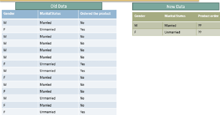
Above problem describes three fields: Gender, Marital Status and whether the product is ordered or not by the customer. Some customers are male and some are female, some customers are married and some are unmarried. Now we have to decide if the customer is Male and if married will he order the Product or not? At the same time we also need to decide if the person is female and if she is unmarried will she order the product or not? Using the historical data if someone has higher probability to order the product then we might sent a different message, if one customer has very low probability to order then we will send a message with discount to attract them to buy the product. If the customer has already higher probability then we will try to do upselling by sending other discounts or cross selling by showing them a different product so that they can buy 2 products. In this way we can improve our business. For solving the problem we have to rearrange the data

Re-Arranging the data

Observations

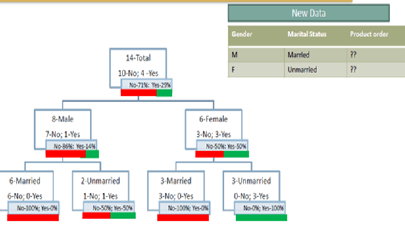
From the above result we have noticed that there are total 14 customers. Among these 14 customers 10 customers did not order the product and 4 have ordered the product. Among these 14 customers there are 8 Males and 6 Females. Among these 8 Males 6 are married and 2 are Unmarried. One married (Male) and one unmarried (Male) have ordered the product.Among 6 Females 3 are married and 3 are unmarried. All unmarried females have ordered the product whereas married females did not ordered the product. This analysis clearly shows that females who are unmarried have high probability to buy the product whereas married females are not interested to buy the product. On the other side Males who are married are not interested to buy the product whereas 50% of Males who are Unmarried are interested to buy the product Therefore,

      Married Males won't buy the product whereas 

      Unmarried Females will buy the product

Decision Tree Approach

Aim is to divide the dataset into segments. Each segment need to be useful for business decision making that means the segment should be pure that means if we segment the whole population into 2 groups, in one group there should be buyers and in the other group there should be non-buyers then we can send different messages related to buyers and non-buyers

Example Sales Segmentation Based on Age

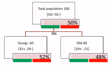
Observations

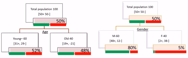
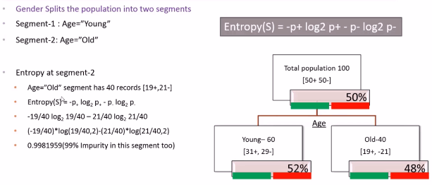
Let us consider there are 100 customers to start with now if we divide these 100 customers based on Age we will get two segments: Young and Old. From the above picture we have noticed that in Young Segment there are 60 People whereas in Old Segment there are 40 People. Now within this 60 Young people 31 are buying and 29 are not buying. Within these old customers 19 are buying and 21 are not buying. At the overall level we came to know that 50% is buying and 50% is not buying which includes both Young and Old.Even if we divide the young customers based on Age it looks like 50% buying and 50% not buying. Again in old customers 50% buying and 50% not buying, then dividing the whole population based on Age doesn’t really help us. Now let us try dividing the whole population based on Gender. Let us see whether this attribute will be helpful in splitting the whole population in a better way or not

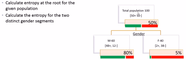
Example Sales Segmentation based on Gender

Observations

Here the whole population is divided into two segments(Male and Female) based on Gender.There are “60” Male customers and “40” Female customers. Within Male customers(60) “48” are buying and “12” are not buying. within Female customers(40) “2” are buying and “38” are not buying.If we see overall out of 50 customers who bought that product 48 are actually Male and only 2 are Female. Within Male there is 80% chance of buying and within female there is only 5% chance of buying. Now when we divide the whole population based on Gender then we can make really good business inferences. Here most of the buyers are Male customers and Non-buyers are female customers. So, dividing the whole population based on Gender is actually giving us a beter split or giving us a better intuition to run a business strategy

Splitting Criterion

The best split is the split that does the best job for separating data into groups whereas each group has very dominant single class that means if we divide the whole population into groups, One group should have entire buyers and one group should have non-buyers.Let us clearly see this concept through Sales segmentation based on AGE as well as through Sales segmentation based on Gender.

Based on AGE

Observations

At root level there is 50% chance of buying and 50% chance of non-buying. Now after the split 52% is positive and 48% is negative in young group whereas in old group 52% is negative and 48% is positive. This is not really giving us pure splits because we did not gain any information really here. At the root level there are 100 customers 50% buying and 50% not buying, even at the split level young and old customer segments both are having 50% chance of buying and 50% chance of not buying. So this AGE variable is not really a good splitting variable.

Based on Gender

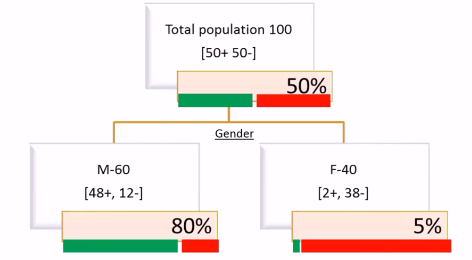
Observations

At root level again 50% chance of buying and 50% chance of non-buying but at the individual splits Male Population has 80% chance of buying whereas female population has only 5% chance of buying that means 95% of female population are not interested to buy the product that is also pure segment from the point of not buying. Male Population is also pure segment from the point of buying. So this split is very much better than eariler split which we have done based on AGE.So we are looking for varibles like GENDER

Impurity or Diversity Measures

Impurity or Diversity Measures gives high score for the AGE variable(high impurity while segmenting),low score for GENDER variable(Low impurity while segmenting) pure segments.

For calculating the impurity there is a mathematical formula called Entropy.

Entropy

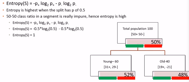
Entropy characterizes the impurity/diversity of a segment. So finally the impurity measure that we are looking is Entropy.Entropyis a measure of uncertainty/impurity/diversity. It measures the information amount in a message. If S is the segment of training measures then

 Entropy(S) = -p+ log2 p+ - p- log2 p-
 
 Where
 
      p+ is the probability of positive class and
 
      p- is the probability of negative class 
 
 Entropy is highest when the split has p of 0.5
 Entropy is least when the split is pure .ie p of 1

Note

If entropy is low we will get better segmentation If entropy is high we will not get better segmentation

Entropy is highest when split has p of 0.5

Entropy is least when split is pure .ie p of 1

Entropy Calculation

LAB: Entropy Calculation – Example

Code – Entropy calculation

Information Gain

Information Gain gives us better picture about the variable based on its splitting criterion. It also provides information before and after the segmentation

    Information Gain= entropy Before Split - entropy After Split 
                           or
  Info gain= (overall entropy at parent node) - (sum of weighted entropy at each child node)

Attribute with maximum Information Gain is best split attribute

Information Gain Calculation

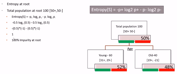
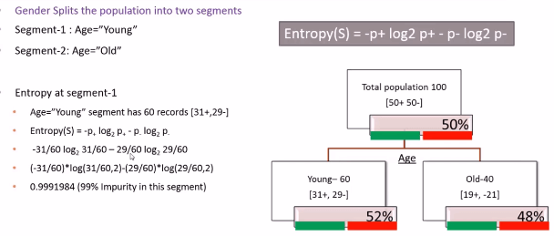
Now lets see how to calculate the Information Gain. we have the overall population(100) at root level and now we have divided the population into two segments:Young and Old based on Age. Each segment has their own Entropies. Entropy at root level is 100%. 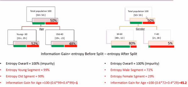From the above picture we observed that Information Gain for variable AGE is very low when compared with the Information Gain of variable GENDER

Lab – Information Gain

Purity or Diversity Measures

There are four Purity or diversity Measures. They are

 Chi-square measure of association
 Information Gain Ratio 
 Classification error
 Gini Index

Decision Tree Algorithm

Major step is to identify the best split variables and best split criteria. Once we have the split then we have to go to segment level and drill down further. In order to find the best attribute for segmentation we will calculate Information Gain for all attributes. The one with the highest attribute is selected

Algorithm

Select a leaf node
Find the best splitting attribute
Spilt the node using the attribute
Go to each child node and repeat step 2 & 3

Stopping criteria

Each leaf-node contains examples of one type
Algorithm ran out of attributes
No further significant information gain

Explanation of the Algorithm

Start with leaf node and then find the best splitting attribute among multiple attributes.Best splitting attribute can be found based on the Information Gain. The one with the highest Information Gain will be the best splitting attribute.After finding the attribute split the node into segments until no further information came

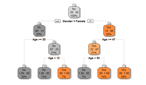
Example

Observations

In the above picture Population is the leaf node. This leaf node is divided into two attributes. Gender and Marital Status. For this two attributes we will calculte Information Gain. The attribute with high Information Gain will be selected for Segmentation.

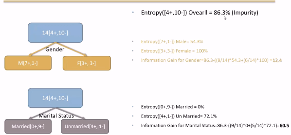
Observations

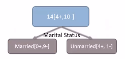
Here we have two attributes GENDER and Marital Status.In order to find the best splitting attribute Information Gain should be calculated for the two attributes.From the above results we clearly noticed that Information Gain for Marital Status is very high when compared with the Information Gain of GENDER variable.Therefore we consider Marital Status attribute and segment the whole population.

Many Splits for a single variable

Sometimes we may find multiple values taken by a variable which will lead to multiple split options for a single variable that will give us multiple information gain values for a single variable.

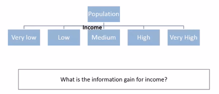
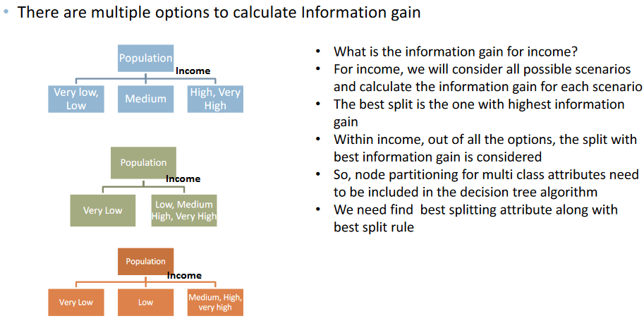
So, in the Decision Tree Algorithm we not only need to find the best variable, we also need to find the best split within that given variable. So, our algorithm for decision tree is slightly modified.

Modified Decision Tree Algorithm

Select a leaf node
Select an attribute -Partition the node population and calculate information gain.
- Find the split with maximum information gain for an attribute
Repeat this for all attributes
- Find the best splitting attribute along with best split rule
Spilt the node using the attribute
Go to each child node and repeat step 2 to 4

Stopping criteria:

Each leaf-node contains examples of one type
Algorithm ran out of attributes
No further significant information gain

Explanation of the Algorithm

We will select one attribute at a time. For each attribute we will calculate the node calculation and we consider all the scenarios and we find the best split criteria then we will have the Information Gain for that particular variable along with the best split criteria and then we do the same thing for all the variables. At the end we will have best splitting Attribute along with best split rule.

LAB: Decision Tree Building

Import Data:Ecom_Cust_Relationship_Management/Ecom_Cust_Survey.csv
How many customers have participated in the survey?
Overall most of the customers are satisfied or dis-satisfied?
Can you segment the data and find the concentrated satisfied and dis-satisfied customer segments ?
What are the major characteristics of satisfied customers?
What are the major characteristics of dis-satisfied customers?

Solution

Import Data:Ecom_Cust_Relationship_Management/Ecom_Cust_Survey.csv

Ecom_Cust_Survey <- read.csv("~DatasetsEcom_Cust_Survey.csv")

How many customers have participated in the survey?

nrow(Ecom_Cust_Survey)

## [1] 11812

Overall most of the customers are satisfied or dis-satisfied?

table(Ecom_Cust_Survey$Overall_Satisfaction)

## 
## Dis Satisfied     Satisfied 
##          6411          5401

Code-Decision Tree Building

rpart(formula, method, data, control)

Formula : y~x1+x2+x3
method: “Class” for classification trees , “anova” for regression trees with continuous output
For controlling tree growth. For example, control=rpart.control(minsplit=30, cp=0.001)
Minsplit : Minimum number of observations in a node be 30 before attempting a split
A split must decrease the overall lack of fit by a factor of 0.001 (cost complexity factor) before being attempted.(details later)
Need the library rpart

library(rpart)

Building Tree Model

Ecom_Tree<-rpart(Overall_Satisfaction~Region+ Age+ Order.Quantity+Customer_Type+Improvement.Area, method="class", data=Ecom_Cust_Survey)
Ecom_Tree

## n= 11812 
## 
## node), split, n, loss, yval, (yprob)
##       * denotes terminal node
## 
## 1) root 11812 5401 Dis Satisfied (0.542753132 0.457246868)  
##   2) Order.Quantity< 40.5 7404 1027 Dis Satisfied (0.861291194 0.138708806)  
##     4) Age>=29.5 7025  652 Dis Satisfied (0.907188612 0.092811388) *
##     5) Age< 29.5 379    4 Satisfied (0.010554090 0.989445910) *
##   3) Order.Quantity>=40.5 4408   34 Satisfied (0.007713249 0.992286751) *

Plotting the Trees

plot(Ecom_Tree, uniform=TRUE)
text(Ecom_Tree, use.n=TRUE, all=TRUE)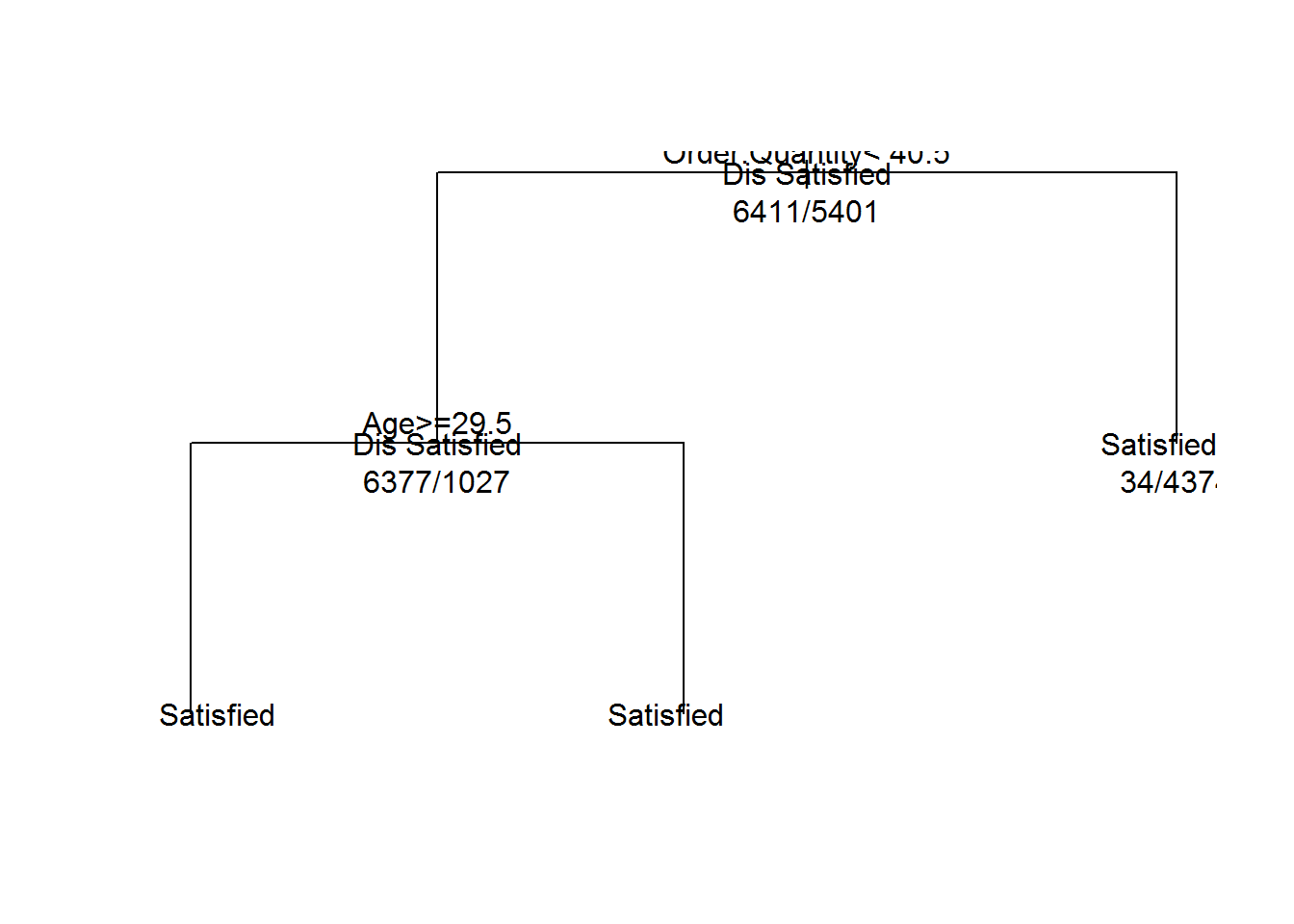

A better looking tree

library(rpart.plot)

## Warning: package 'rpart.plot' was built under R version 3.3.2

prp(Ecom_Tree,box.col=c("Grey", "Orange")[Ecom_Tree$frame$yval],varlen=0, type=1,extra=4,under=TRUE)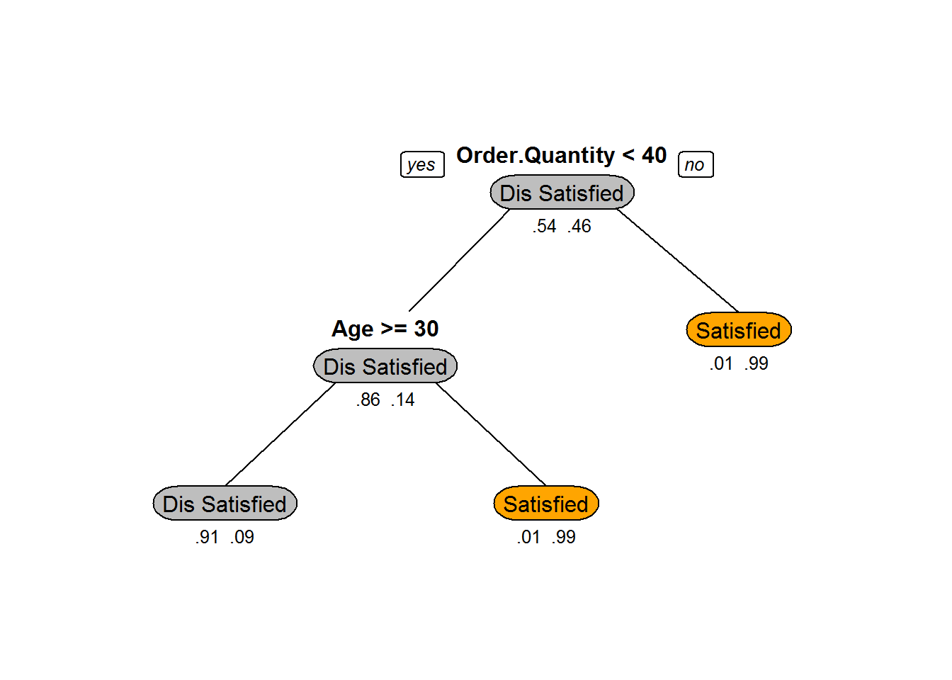

Tree Validation

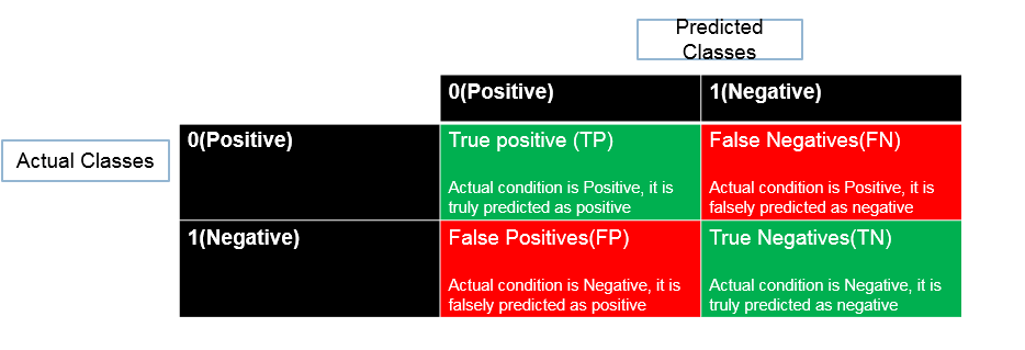
Accuracy=(TP+TN)/(TP+FP+FN+TN)
Misclassification Rate=(FP+FN)/(TP+FP+FN+TN)

LAB: Tree Validation

Find the accuracy of the classification for the Ecom_Cust_Survey model

predicted_values<-predict(Ecom_Tree,type="class")
actual_values<-Ecom_Cust_Survey$Overall_Satisfaction

conf_matrix<-table(predicted_values,actual_values)
conf_matrix

##                 actual_values
## predicted_values Dis Satisfied Satisfied
##    Dis Satisfied          6373       652
##    Satisfied                38      4749

accuracy<-(conf_matrix[1,1]+conf_matrix[2,2])/(sum(conf_matrix))
accuracy

## [1] 0.9415848

LAB: The Problem of Over-fitting

Import Dataset: “Buyers Profiles/Train_data.csv”
Import both test and training data
Build a decision tree model on training data
Find the accuracy on training data
Find the predictions for test data
What is the model prediction accuracy on test data?

Solution

Import Dataset: “Buyers Profiles/Train_data.csv”
Import both test and training data

Train <- read.csv("H:studiesDATA ANALYTICS2.Machine Learning AlgorithmsDecision TreesDatasetsTrain_data.csv")
Test <- read.csv("H:studiesDATA ANALYTICS2.Machine Learning AlgorithmsDecision TreesDatasetsTest_data.csv")

Build a decision tree model on training data

buyers_model<-rpart(Bought ~ Age + Gender, method="class", data=Train,control=rpart.control(minsplit=2))
buyers_model

## n= 14 
## 
## node), split, n, loss, yval, (yprob)
##       * denotes terminal node
## 
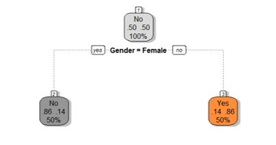
##  1) root 14 7 No (0.5000000 0.5000000)  
##    2) Gender=Female 7 1 No (0.8571429 0.1428571)  
##      4) Age>=20 4 0 No (1.0000000 0.0000000) *
##      5) Age< 20 3 1 No (0.6666667 0.3333333)  
##       10) Age< 11.5 2 0 No (1.0000000 0.0000000) *
##       11) Age>=11.5 1 0 Yes (0.0000000 1.0000000) *
##    3) Gender=Male 7 1 Yes (0.1428571 0.8571429)  
##      6) Age>=47 3 1 Yes (0.3333333 0.6666667)  
##       12) Age< 52 1 0 No (1.0000000 0.0000000) *
##       13) Age>=52 2 0 Yes (0.0000000 1.0000000) *
##      7) Age< 47 4 0 Yes (0.0000000 1.0000000) *

Find the accuracy on training data

predicted_values<-predict(buyers_model,type="class")
actual_values<-Train$Bought

conf_matrix<-table(predicted_values,actual_values)
accuracy<-(conf_matrix[1,1]+conf_matrix[2,2])/(sum(conf_matrix))
accuracy

## [1] 1

Find the predictions for test data

predicted_values<-predict(buyers_model,type="class",newdata=Test)
predicted_values

##   1   2   3   4   5   6 
##  No  No  No Yes  No Yes 
## Levels: No Yes

What is the model prediction accuracy on test data?

actual_values<-Test$Bought

conf_matrix<-table(predicted_values,actual_values)
accuracy<-(conf_matrix[1,1]+conf_matrix[2,2])/(sum(conf_matrix))
accuracy

## [1] 0.3333333

The Final Tree with Rules

1. Gender=Female & Age>=20 No *
1. Gender=Female & Age< 20 & Age< 11.5 No *
1. Gender=Female & Age< 20 & Age>=11.5 Yes *
1. Gender=Male & Age>=47 & Age< 52 No *
1. Gender=Male & Age>=47 & Age>=52 Yes *
1. Gender=Male & Age< 47 Yes *

The Problem of Overfitting

If we further grow the tree we might even see each row of the input data table as the final rules
The model will be really good on the training data but it will fail to validate on the test data
Growing the tree beyond a certain level of complexity leads to overfitting
A really big tree is very likely to suffer from overfitting.

Pruning

Growing the tree beyond a certain level of complexity leads to overfitting
In our data, age doesn’t have any impact on the target variable.
Growing the tree beyond Gender is not going to add any value. Need to cut it at Gender
This process of trimming trees is called Pruning

buyers_model1<-rpart(Bought ~ Gender, method="class", data=Train,control=rpart.control(minsplit=2))
prp(buyers_model1,box.col=c("Grey", "Orange")[buyers_model1$frame$yval],varlen=0,faclen=0, type=1,extra=4,under=TRUE)

Pruning to Avoid Overfitting

Pruning helps us to avoid overfitting
Generally it is preferred to have a simple model, it avoids overfitting issue
Any additional split that does not add significant value is not worth while.
We can use Cp – Complexity parameter in R to control the tree growth

Complexity Parameter

Complexity parameter is used to mention the minimum improvement before proceeding further.
It is the amount by which splitting a node improved the relative error.
For example, in a decision tree, before splitting the node, the error is 0.5 and after splitting the error is 0.1 then the split is useful, where as if the error before splitting is 0.5 and after splitting it is 0.48 then split didn’t really help
User tells the program that any split which does not improve the fit by cp will likely be pruned off
This can be used as a good stopping criterion.
The main role of this parameter is to avoid overfitting and also to save computing time by pruning off splits that are obviously not worthwhile
It is similar to Adj R-square. If a variable doesn’t have a significant impact then there is no point in adding it. If we add such variable adj R square decreases.
The default is of cp is 0.01.

Code-Tree Pruning and Complexity Parameter

Sample_tree<-rpart(Bought~Gender+Age, method="class", data=Train, control=rpart.control(minsplit=2, cp=0.001))
Sample_tree

## n= 14 
## 
## node), split, n, loss, yval, (yprob)
##       * denotes terminal node
## 
##  1) root 14 7 No (0.5000000 0.5000000)  
##    2) Gender=Female 7 1 No (0.8571429 0.1428571)  
##      4) Age>=20 4 0 No (1.0000000 0.0000000) *
##      5) Age< 20 3 1 No (0.6666667 0.3333333)  
##       10) Age< 11.5 2 0 No (1.0000000 0.0000000) *
##       11) Age>=11.5 1 0 Yes (0.0000000 1.0000000) *
##    3) Gender=Male 7 1 Yes (0.1428571 0.8571429)  
##      6) Age>=47 3 1 Yes (0.3333333 0.6666667)  
##       12) Age< 52 1 0 No (1.0000000 0.0000000) *
##       13) Age>=52 2 0 Yes (0.0000000 1.0000000) *
##      7) Age< 47 4 0 Yes (0.0000000 1.0000000) *

Sample_tree_1<-rpart(Bought~Gender+Age, method="class", data=Train, control=rpart.control(minsplit=2, cp=0.1))
Sample_tree_1

## n= 14 
## 
## node), split, n, loss, yval, (yprob)
##       * denotes terminal node
## 
## 1) root 14 7 No (0.5000000 0.5000000)  
##   2) Gender=Female 7 1 No (0.8571429 0.1428571) *
##   3) Gender=Male 7 1 Yes (0.1428571 0.8571429) *

The default is 0.01.

Choosing Cp and Cross Validation Error

We can choose Cp by analyzing the cross validation error.
For every split we expect the validation error to reduce, but if the model suffers from overfitting the cross validation error increases or shows negligible improvement
We can either rebuild the tree with updated cp or prune the already built tree by mentioning the old tree and new cp value
printcp(tree) shows the
Training error , cross validation error and standard deviation at each node.

Code – Choosing Cp

Cp display the results

printcp(Sample_tree)

## 
## Classification tree:
## rpart(formula = Bought ~ Gender + Age, data = Train, method = "class", 
##     control = rpart.control(minsplit = 2, cp = 0.001))
## 
## Variables actually used in tree construction:
## [1] Age    Gender
## 
## Root node error: 7/14 = 0.5
## 
## n= 14 
## 
##         CP nsplit rel error  xerror    xstd
## 1 0.714286      0   1.00000 1.57143 0.21933
## 2 0.071429      1   0.28571 0.28571 0.18704
## 3 0.001000      5   0.00000 0.57143 0.24147

Code – Cross Validation Error

cross-validation results

plotcp(Sample_tree)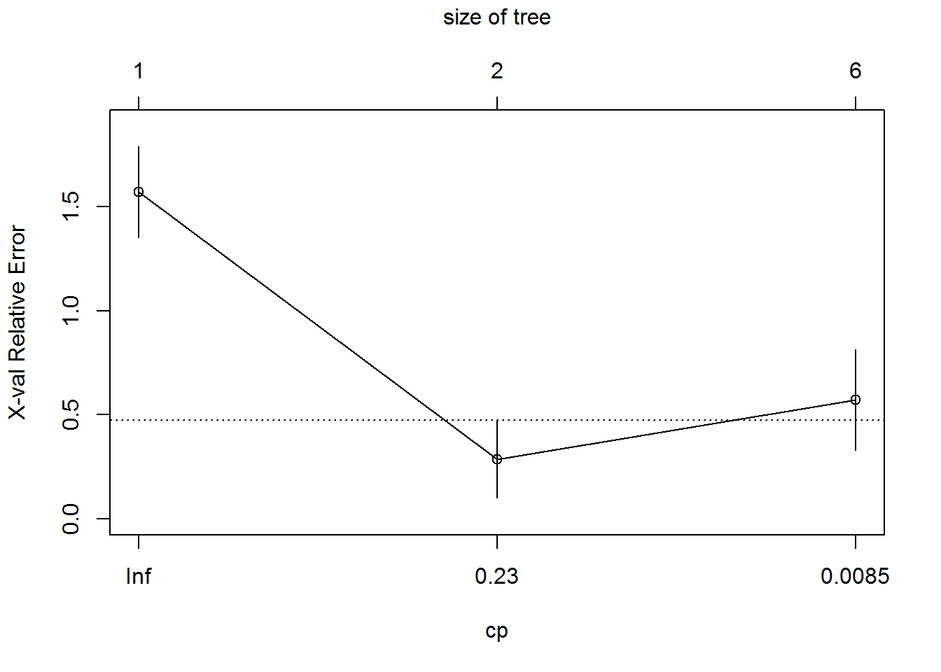

New Model with Selected Cp

Sample_tree_2<-rpart(Bought~Gender+Age, method="class", data=Train, control=rpart.control(minsplit=2, cp=0.23))
Sample_tree_2

## n= 14 
## 
## node), split, n, loss, yval, (yprob)
##       * denotes terminal node
## 
## 1) root 14 7 No (0.5000000 0.5000000)  
##   2) Gender=Female 7 1 No (0.8571429 0.1428571) *
##   3) Gender=Male 7 1 Yes (0.1428571 0.8571429) *

Plotting the Tree

prp(Sample_tree_2,box.col=c("Grey", "Orange")[Sample_tree_2$frame$yval],varlen=0,faclen=0, type=1,extra=4,under=TRUE)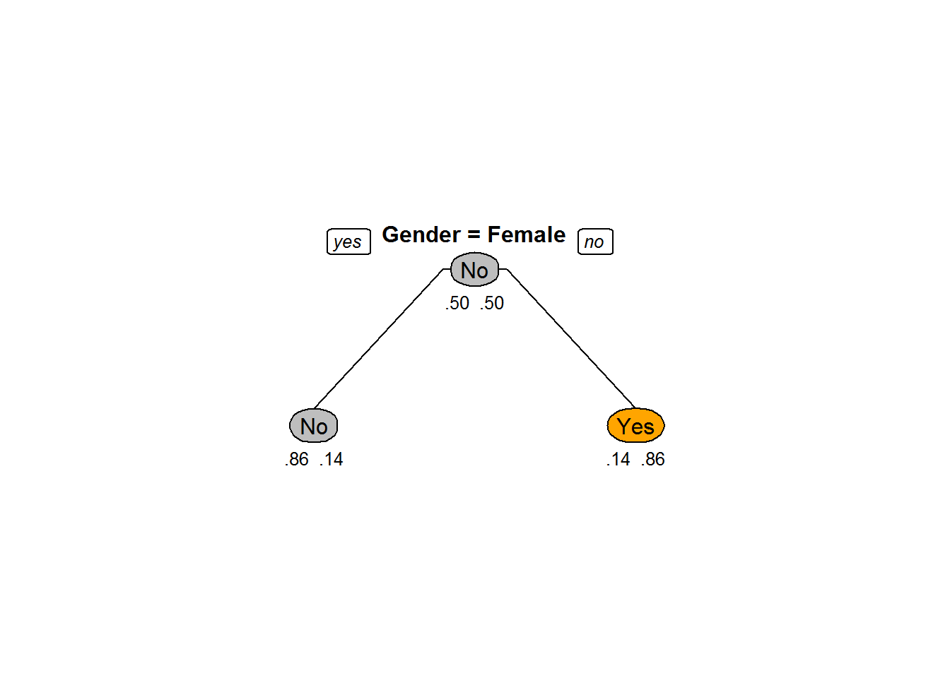

Post Pruning the Old Tree

Pruned_tree<-prune(Sample_tree,cp=0.23)
prp(Pruned_tree,box.col=c("Grey", "Orange")[Sample_tree$frame$yval],varlen=0,faclen=0, type=1,extra=4,under=TRUE)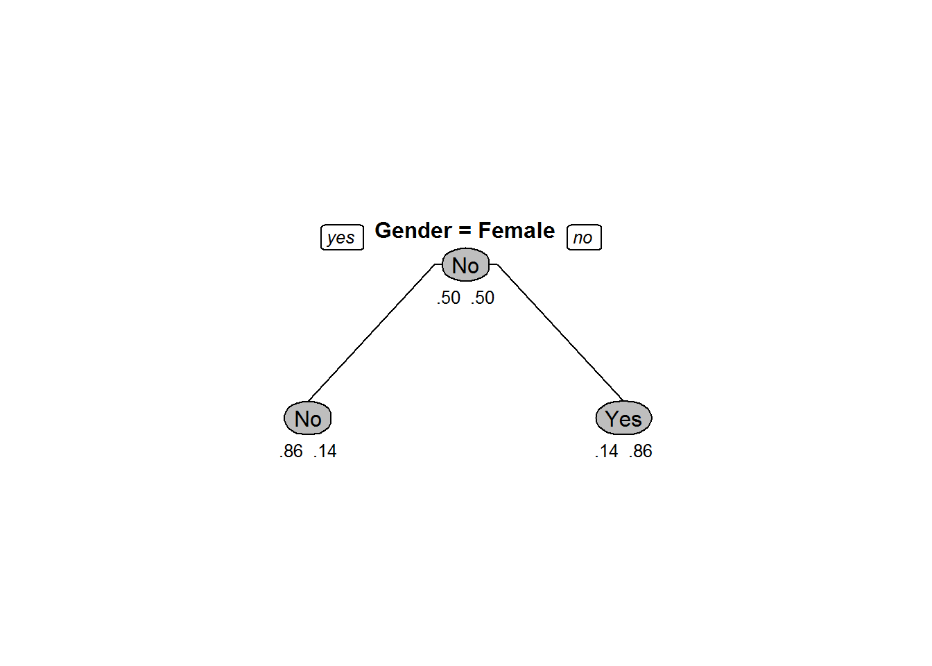

Code-Choosing Cp

Ecom_Tree<-rpart(Overall_Satisfaction~Region+ Age+ Order.Quantity+Customer_Type+Improvement.Area, method="class", control=rpart.control(minsplit=30,cp=0.001),data=Ecom_Cust_Survey)
printcp(Ecom_Tree)

## 
## Classification tree:
## rpart(formula = Overall_Satisfaction ~ Region + Age + Order.Quantity + 
##     Customer_Type + Improvement.Area, data = Ecom_Cust_Survey, 
##     method = "class", control = rpart.control(minsplit = 30, 
##         cp = 0.001))
## 
## Variables actually used in tree construction:
## [1] Age              Customer_Type    Improvement.Area Order.Quantity  
## [5] Region          
## 
## Root node error: 5401/11812 = 0.45725
## 
## n= 11812 
## 
##          CP nsplit rel error  xerror      xstd
## 1 0.8035549      0   1.00000 1.00000 0.0100245
## 2 0.0686910      1   0.19645 0.19645 0.0057537
## 3 0.0029624      2   0.12775 0.12775 0.0047193
## 4 0.0022218      5   0.11887 0.12757 0.0047161
## 5 0.0018515      7   0.11442 0.12090 0.0045987
## 6 0.0014812      8   0.11257 0.11627 0.0045148
## 7 0.0010000      9   0.11109 0.11739 0.0045351

Code-Choosing Cp

plotcp(Ecom_Tree)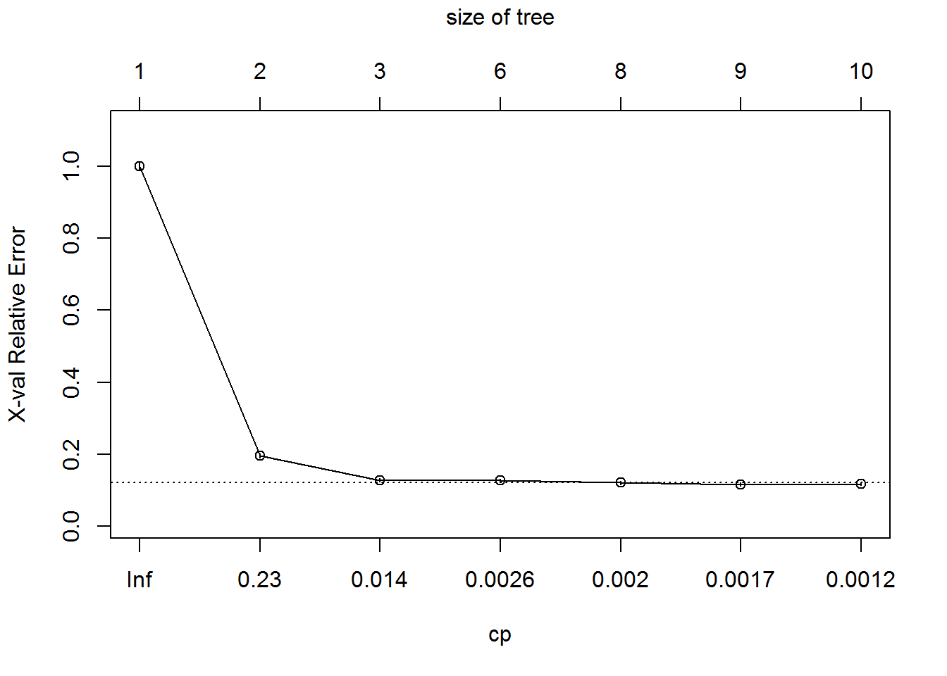

– Choose Cp as 0.0029646

Code – Pruning

Ecom_Tree_prune<-prune(Ecom_Tree,cp=0.0029646)
Ecom_Tree_prune

## n= 11812 
## 
## node), split, n, loss, yval, (yprob)
##       * denotes terminal node
## 
## 1) root 11812 5401 Dis Satisfied (0.542753132 0.457246868)  
##   2) Order.Quantity< 40.5 7404 1027 Dis Satisfied (0.861291194 0.138708806)  
##     4) Age>=29.5 7025  652 Dis Satisfied (0.907188612 0.092811388) *
##     5) Age< 29.5 379    4 Satisfied (0.010554090 0.989445910) *
##   3) Order.Quantity>=40.5 4408   34 Satisfied (0.007713249 0.992286751) *

Plot – Beofre and After Pruning

prp(Ecom_Tree,box.col=c("Grey", "Orange")[Ecom_Tree$frame$yval],varlen=0,faclen=0, type=1,extra=4,under=TRUE)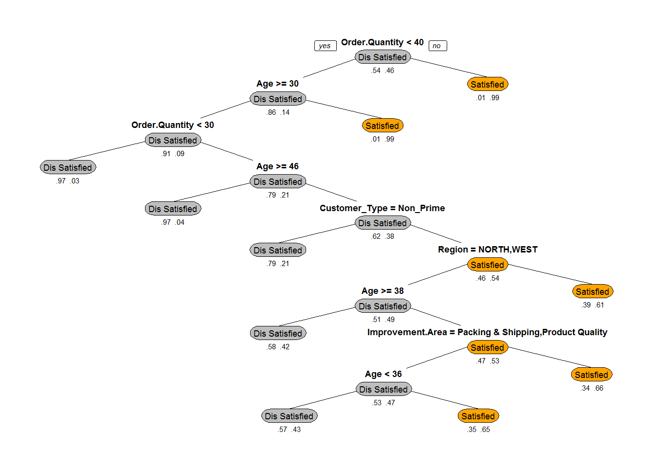

***

prp(Ecom_Tree_prune,box.col=c("Grey", "Orange")[Ecom_Tree$frame$yval],varlen=0,faclen=0, type=1,extra=4,under=TRUE)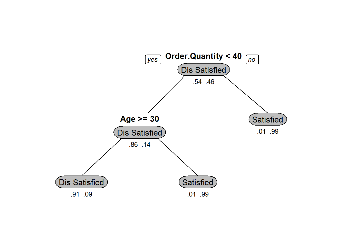

Two Types of Pruning

Pre-Pruning:
Building the tree by mentioning Cp value upfront
Post-pruning:
Grow decision tree to its entirety, trim the nodes of the decision tree in a bottom-up fashion

LAB: Tree Building & Model Selection

Import fiber bits data. This is internet service provider data. The idea is to predict the customer attrition based on some independent factors
Build a decision tree model for fiber bits data
Prune the tree if required
Find out the final accuracy
Is there any 100% active/inactive customer segment?

Solution

Fiberbits <- read.csv("~DatasetsFiberbits.csv")
Fiber_bits_tree<-rpart(active_cust~., method="class", control=rpart.control(minsplit=30, cp=0.001), data=Fiberbits)
Fiber_bits_tree

## n= 100000 
## 
## node), split, n, loss, yval, (yprob)
##       * denotes terminal node
## 
##    1) root 100000 42141 1 (0.42141000 0.57859000)  
##      2) relocated>=0.5 12348   954 0 (0.92274052 0.07725948)  
##        4) technical_issues_per_month>=1.5 11294   526 0 (0.95342660 0.04657340) *
##        5) technical_issues_per_month< 1.5 1054   428 0 (0.59392789 0.40607211)  
##         10) number_plan_changes>=4.5 495    45 0 (0.90909091 0.09090909) *
##         11) number_plan_changes< 4.5 559   176 1 (0.31484794 0.68515206)  
##           22) Speed_test_result< 79.5 45     0 0 (1.00000000 0.00000000) *
##           23) Speed_test_result>=79.5 514   131 1 (0.25486381 0.74513619) *
##      3) relocated< 0.5 87652 30747 1 (0.35078492 0.64921508)  
##        6) Speed_test_result< 78.5 27517 10303 0 (0.62557692 0.37442308)  
##         12) technical_issues_per_month>=3.5 22187  5791 0 (0.73899130 0.26100870)  
##           24) number_plan_changes< 0.5 9735  1132 0 (0.88371854 0.11628146)  
##             48) Speed_test_result< 77.5 7750   541 0 (0.93019355 0.06980645) *
##             49) Speed_test_result>=77.5 1985   591 0 (0.70226700 0.29773300)  
##               98) income>=2008.5 1211   133 0 (0.89017341 0.10982659)  
##                196) income< 2526 1163    85 0 (0.92691316 0.07308684) *
##                197) income>=2526 48     0 1 (0.00000000 1.00000000) *
##               99) income< 2008.5 774   316 1 (0.40826873 0.59173127)  
##                198) income< 1785.5 270    97 0 (0.64074074 0.35925926) *
##                199) income>=1785.5 504   143 1 (0.28373016 0.71626984) *
##           25) number_plan_changes>=0.5 12452  4659 0 (0.62584324 0.37415676)  
##             50) number_plan_changes>=1.5 7867  1358 0 (0.82738020 0.17261980) *
##             51) number_plan_changes< 1.5 4585  1284 1 (0.28004362 0.71995638) *
##         13) technical_issues_per_month< 3.5 5330   818 1 (0.15347092 0.84652908)  
##           26) income>=1945.5 1849   619 1 (0.33477555 0.66522445)  
##             52) monthly_bill>=148 167    29 0 (0.82634731 0.17365269) *
##             53) monthly_bill< 148 1682   481 1 (0.28596908 0.71403092)  
##              106) income< 2362 1407   472 1 (0.33546553 0.66453447)  
##                212) technical_issues_per_month>=1.5 176    25 0 (0.85795455 0.14204545) *
##                213) technical_issues_per_month< 1.5 1231   321 1 (0.26076361 0.73923639)  
##                  426) income>=2180.5 126    21 0 (0.83333333 0.16666667) *
##                  427) income< 2180.5 1105   216 1 (0.19547511 0.80452489) *
##              107) income>=2362 275     9 1 (0.03272727 0.96727273) *
##           27) income< 1945.5 3481   199 1 (0.05716748 0.94283252) *
##        7) Speed_test_result>=78.5 60135 13533 1 (0.22504365 0.77495635)  
##         14) Speed_test_result< 82.5 25734  9271 1 (0.36026269 0.63973731)  
##           28) Speed_test_result>=80.5 11671  5312 0 (0.54485477 0.45514523)  
##             56) income>=1722.5 6306  1299 0 (0.79400571 0.20599429)  
##              112) income< 1992.5 5828   888 0 (0.84763212 0.15236788)  
##                224) number_plan_changes>=1.5 3053   189 0 (0.93809368 0.06190632) *
##                225) number_plan_changes< 1.5 2775   699 0 (0.74810811 0.25189189)  
##                  450) number_plan_changes< 0.5 2284   358 0 (0.84325744 0.15674256)  
##                    900) technical_issues_per_month>=3.5 1511    57 0 (0.96227664 0.03772336) *
##                    901) technical_issues_per_month< 3.5 773   301 0 (0.61060802 0.38939198)  
##                     1802) monthly_bill>=148 364    41 0 (0.88736264 0.11263736) *
##                     1803) monthly_bill< 148 409   149 1 (0.36430318 0.63569682) *
##                  451) number_plan_changes>=0.5 491   150 1 (0.30549898 0.69450102) *
##              113) income>=1992.5 478    67 1 (0.14016736 0.85983264) *
##             57) income< 1722.5 5365  1352 1 (0.25200373 0.74799627)  
##              114) number_plan_changes>=1.5 1586   680 1 (0.42875158 0.57124842)  
##                228) Speed_test_result< 81.5 894   370 0 (0.58612975 0.41387025)  
##                  456) technical_issues_per_month>=3.5 301    54 0 (0.82059801 0.17940199) *
##                  457) technical_issues_per_month< 3.5 593   277 1 (0.46711636 0.53288364)  
##                    914) income< 1604.5 261    92 0 (0.64750958 0.35249042) *
##                    915) income>=1604.5 332   108 1 (0.32530120 0.67469880) *
##                229) Speed_test_result>=81.5 692   156 1 (0.22543353 0.77456647) *
##              115) number_plan_changes< 1.5 3779   672 1 (0.17782482 0.82217518) *
##           29) Speed_test_result< 80.5 14063  2912 1 (0.20706819 0.79293181)  
##             58) income< 1960.5 11360  2725 1 (0.23987676 0.76012324)  
##              116) Num_complaints>=4.5 292    87 0 (0.70205479 0.29794521)  
##                232) technical_issues_per_month>=3.5 197     0 0 (1.00000000 0.00000000) *
##                233) technical_issues_per_month< 3.5 95     8 1 (0.08421053 0.91578947) *
##              117) Num_complaints< 4.5 11068  2520 1 (0.22768341 0.77231659)  
##                234) number_plan_changes>=1.5 4003  1180 1 (0.29477892 0.70522108)  
##                  468) income>=1809.5 1229   582 1 (0.47355574 0.52644426)  
##                    936) Speed_test_result>=79.5 477   132 0 (0.72327044 0.27672956) *
##                    937) Speed_test_result< 79.5 752   237 1 (0.31515957 0.68484043) *
##                  469) income< 1809.5 2774   598 1 (0.21557318 0.78442682) *
##                235) number_plan_changes< 1.5 7065  1340 1 (0.18966737 0.81033263) *
##             59) income>=1960.5 2703   187 1 (0.06918239 0.93081761) *
##         15) Speed_test_result>=82.5 34401  4262 1 (0.12389175 0.87610825) *

Plotting the Tree

prp(Fiber_bits_tree,box.col=c("Grey", "Orange")[Fiber_bits_tree$frame$yval],varlen=0,faclen=0, type=1,extra=4,under=TRUE)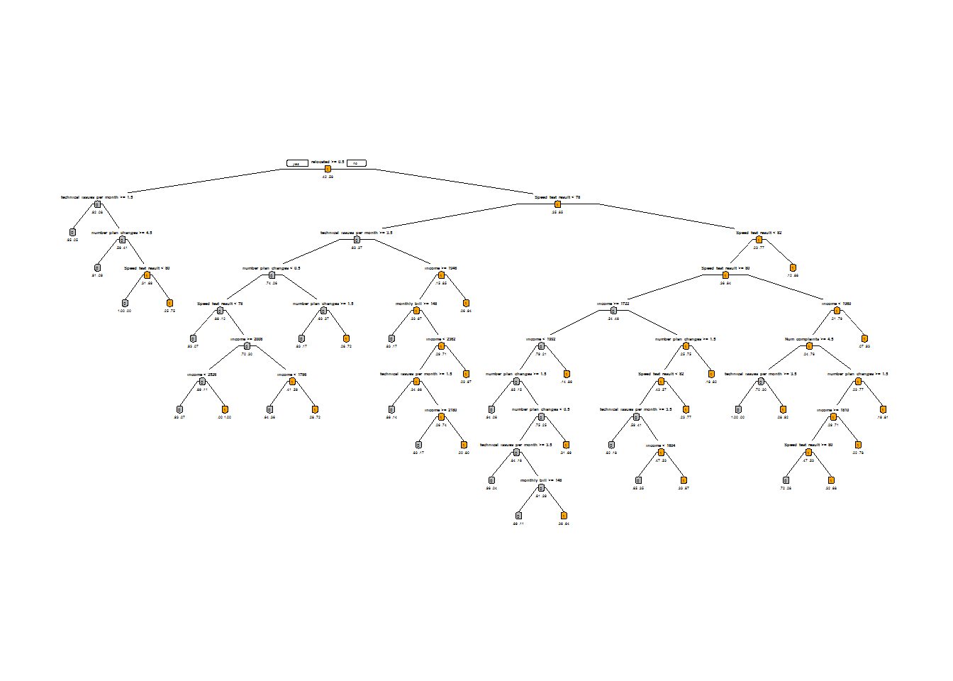

Code-Choosing Cp and Cross Validation Error

printcp(Fiber_bits_tree)

## 
## Classification tree:
## rpart(formula = active_cust ~ ., data = Fiberbits, method = "class", 
##     control = rpart.control(minsplit = 30, cp = 0.001))
## 
## Variables actually used in tree construction:
## [1] income                     monthly_bill              
## [3] Num_complaints             number_plan_changes       
## [5] relocated                  Speed_test_result         
## [7] technical_issues_per_month
## 
## Root node error: 42141/100000 = 0.42141
## 
## n= 100000 
## 
##           CP nsplit rel error  xerror      xstd
## 1  0.2477397      0   1.00000 1.00000 0.0037054
## 2  0.1639971      1   0.75226 0.75226 0.0034917
## 3  0.0876581      2   0.58826 0.58826 0.0032402
## 4  0.0293301      3   0.50061 0.50061 0.0030616
## 5  0.0239316      6   0.41261 0.41307 0.0028453
## 6  0.0081631      8   0.36475 0.37481 0.0027367
## 7  0.0024560      9   0.35659 0.35811 0.0026862
## 8  0.0022662     11   0.35168 0.35407 0.0026737
## 9  0.0018272     13   0.34714 0.34558 0.0026469
## 10 0.0016848     15   0.34349 0.34332 0.0026398
## 11 0.0014001     18   0.33832 0.33953 0.0026276
## 12 0.0013763     24   0.32859 0.33478 0.0026122
## 13 0.0013170     26   0.32583 0.33348 0.0026079
## 14 0.0012933     28   0.32320 0.32892 0.0025929
## 15 0.0011390     33   0.31563 0.32147 0.0025681
## 16 0.0010678     34   0.31449 0.31912 0.0025601
## 17 0.0010000     35   0.31342 0.31779 0.0025556

Plot-Choosing Cp and Cross Validation Error

plotcp(Fiber_bits_tree)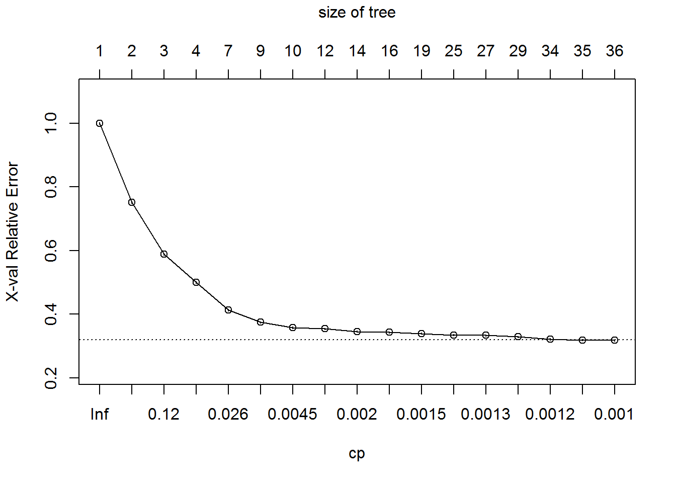

Pruning

Fiber_bits_tree_1<-prune(Fiber_bits_tree, cp=0.0081631)
Fiber_bits_tree_1

## n= 100000 
## 
## node), split, n, loss, yval, (yprob)
##       * denotes terminal node
## 
##  1) root 100000 42141 1 (0.42141000 0.57859000)  
##    2) relocated>=0.5 12348   954 0 (0.92274052 0.07725948) *
##    3) relocated< 0.5 87652 30747 1 (0.35078492 0.64921508)  
##      6) Speed_test_result< 78.5 27517 10303 0 (0.62557692 0.37442308)  
##       12) technical_issues_per_month>=3.5 22187  5791 0 (0.73899130 0.26100870)  
##         24) number_plan_changes< 0.5 9735  1132 0 (0.88371854 0.11628146) *
##         25) number_plan_changes>=0.5 12452  4659 0 (0.62584324 0.37415676)  
##           50) number_plan_changes>=1.5 7867  1358 0 (0.82738020 0.17261980) *
##           51) number_plan_changes< 1.5 4585  1284 1 (0.28004362 0.71995638) *
##       13) technical_issues_per_month< 3.5 5330   818 1 (0.15347092 0.84652908) *
##      7) Speed_test_result>=78.5 60135 13533 1 (0.22504365 0.77495635)  
##       14) Speed_test_result< 82.5 25734  9271 1 (0.36026269 0.63973731)  
##         28) Speed_test_result>=80.5 11671  5312 0 (0.54485477 0.45514523)  
##           56) income>=1722.5 6306  1299 0 (0.79400571 0.20599429) *
##           57) income< 1722.5 5365  1352 1 (0.25200373 0.74799627) *
##         29) Speed_test_result< 80.5 14063  2912 1 (0.20706819 0.79293181) *
##       15) Speed_test_result>=82.5 34401  4262 1 (0.12389175 0.87610825) *

Plot after Pruning

prp(Fiber_bits_tree_1,box.col=c("Grey", "Orange")[Fiber_bits_tree$frame$yval],varlen=0,faclen=0, type=1,extra=4,under=TRUE)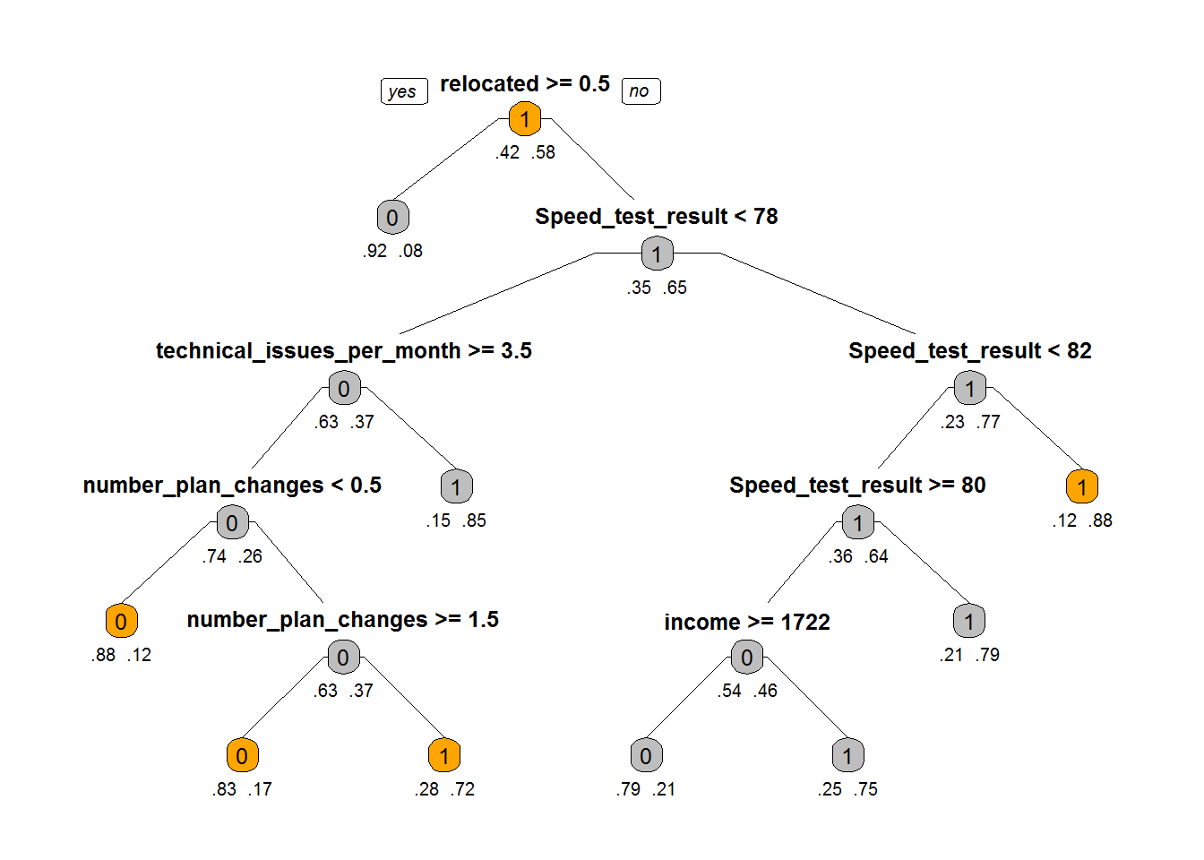

Choosing Cp and Cross Validation Error with New Model

printcp(Fiber_bits_tree_1)

## 
## Classification tree:
## rpart(formula = active_cust ~ ., data = Fiberbits, method = "class", 
##     control = rpart.control(minsplit = 30, cp = 0.001))
## 
## Variables actually used in tree construction:
## [1] income                     number_plan_changes       
## [3] relocated                  Speed_test_result         
## [5] technical_issues_per_month
## 
## Root node error: 42141/100000 = 0.42141
## 
## n= 100000 
## 
##          CP nsplit rel error  xerror      xstd
## 1 0.2477397      0   1.00000 1.00000 0.0037054
## 2 0.1639971      1   0.75226 0.75226 0.0034917
## 3 0.0876581      2   0.58826 0.58826 0.0032402
## 4 0.0293301      3   0.50061 0.50061 0.0030616
## 5 0.0239316      6   0.41261 0.41307 0.0028453
## 6 0.0081631      8   0.36475 0.37481 0.0027367

plotcp(Fiber_bits_tree_1)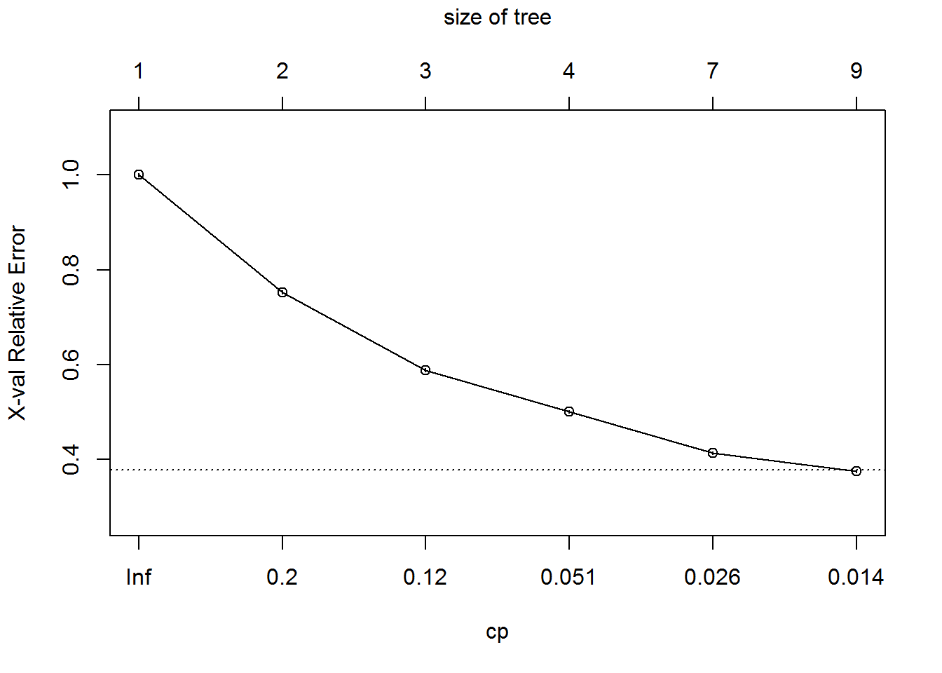

Pruning further

Fiber_bits_tree_2<-prune(Fiber_bits_tree, cp=0.0239316)
Fiber_bits_tree_2

## n= 100000 
## 
## node), split, n, loss, yval, (yprob)
##       * denotes terminal node
## 
##  1) root 100000 42141 1 (0.42141000 0.57859000)  
##    2) relocated>=0.5 12348   954 0 (0.92274052 0.07725948) *
##    3) relocated< 0.5 87652 30747 1 (0.35078492 0.64921508)  
##      6) Speed_test_result< 78.5 27517 10303 0 (0.62557692 0.37442308)  
##       12) technical_issues_per_month>=3.5 22187  5791 0 (0.73899130 0.26100870) *
##       13) technical_issues_per_month< 3.5 5330   818 1 (0.15347092 0.84652908) *
##      7) Speed_test_result>=78.5 60135 13533 1 (0.22504365 0.77495635)  
##       14) Speed_test_result< 82.5 25734  9271 1 (0.36026269 0.63973731)  
##         28) Speed_test_result>=80.5 11671  5312 0 (0.54485477 0.45514523)  
##           56) income>=1722.5 6306  1299 0 (0.79400571 0.20599429) *
##           57) income< 1722.5 5365  1352 1 (0.25200373 0.74799627) *
##         29) Speed_test_result< 80.5 14063  2912 1 (0.20706819 0.79293181) *
##       15) Speed_test_result>=82.5 34401  4262 1 (0.12389175 0.87610825) *

Tree- After Pruning further

prp(Fiber_bits_tree_2,box.col=c("Grey", "Orange")[Fiber_bits_tree$frame$yval],varlen=0,faclen=0, type=1,extra=4,under=TRUE)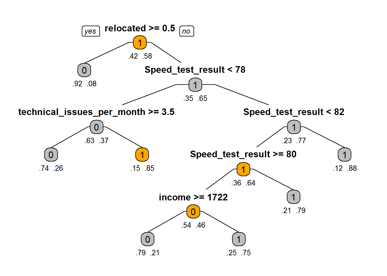

Conclusion

Decision trees are powerful and very simple to represent and understand.
One need to be careful with the size of the tree. Decision trees are more prone to overfitting than other algorithms
Can be applied to any type of data, especially with categorical predictors
One can use decision trees to perform a basic customer segmentation and build a different predictive model on the segments

Problem of Overfitting

Most of the decision trees suffer from a problem called Overfitting.

Pruning

To overcome the problem of Overfitting we need to trim the trees beyond certain level of complexity. This process of trimming trees is called Pruning. Pruning helps us to avoid Overfitting. We can use Cp – Complexity parameter in R to control the tree growth

Complexity Parameter

In R we can set the Complexity parameter to prune the trees or to stop the growth of the trees to avoid Overfitting. Imagine before splitting the node, the error is 0.5 and after splitting the error is 0.1 then the split is useful, where as if the error before splitting is 0.5 and after splitting it is 0.48 then split didn’t really help. In such case we can mention Complexity parameter and we specifically say that if 10% of improvement is not there then do not grow the tree. User tells the program that any split which does not improve the fit by cp will likely be pruned off. This can be used as a good stopping criterion. The main role of this parameter is to avoid Overfitting and also to save computing time by pruning off splits that are obviously not worthwhile. The default is of cp is 0.01.

Observations

From the above results we have noticed that after including Complexity Parameter in Decision Tree modeling the accuracy of testing and training data are very nearer. This shows the avoidance of Overfitting.

Choosing Complexity Parameter and Cross Validation Error

Observations

printcp () is used to print values related to that particular tree. It shows training error, cross validation error and standard deviation at each of the nodes. Cross Validation Error at Root level = 1.71429, Second level = 0.28571 and Third level = 0.71429. Above Cross validation error clearly shows that error has been decreased from Root level to second level whereas from Second level to Third level it has been increased. This clearly indicates that we need to trim third level (as its error is more than 2nd level) and consider the tree up to second level itself. We can see it from the graph. The plot shows that when cp = infinity, error is high ,when cp=0.23 error is around 0.3 and when cp=0.027 error is around 0.7. From these results we can conclude that, it is better to cut the tree at 2nd level as third level has more error than 2nd level so we select cp value of 2nd level. In this way the Complexity Parameter will be chosen.

Types of Pruning

There are 2 types of pruning. They are 1. Pre-Pruning 2. Post-Pruning Pre-Pruning: Building the tree by mentioning Cp value upfront. Post-pruning: Grow decision tree to its entirety, trim the nodes of the decision tree in a bottom-up fashion

Select Category

Handout – Decision Tree in R

You can download the datasets and R code file for this session here.

Introduction

Contents

What is Segmentation?

Segmentation Business Problem

Observations

Re-Arranging the data

Observations

Decision Tree Approach

Example Sales Segmentation Based on Age

Observations

Example Sales Segmentation based on Gender

Observations

Splitting Criterion

Based on AGE

Observations

Based on Gender

Observations

Impurity or Diversity Measures

Entropy

Note

Entropy is highest when split has p of 0.5

Entropy is least when split is pure .ie p of 1

Entropy Calculation

LAB: Entropy Calculation – Example

Code – Entropy calculation

Information Gain

Information Gain Calculation

Lab – Information Gain

Purity or Diversity Measures

Decision Tree Algorithm

Algorithm

Stopping criteria

Explanation of the Algorithm

Example

Observations

Observations

Many Splits for a single variable

Modified Decision Tree Algorithm

Stopping criteria:

Explanation of the Algorithm

LAB: Decision Tree Building

Solution

Code-Decision Tree Building

Plotting the Trees

A better looking tree

Tree Validation

LAB: Tree Validation

LAB: The Problem of Over-fitting

Solution

The Final Tree with Rules

The Problem of Overfitting

Pruning

Pruning to Avoid Overfitting

Complexity Parameter

Code-Tree Pruning and Complexity Parameter

Choosing Cp and Cross Validation Error

Code – Choosing Cp

Code – Cross Validation Error

New Model with Selected Cp

Plotting the Tree

Post Pruning the Old Tree

Code-Choosing Cp

Code – Pruning

Plot – Beofre and After Pruning

Two Types of Pruning

LAB: Tree Building & Model Selection

Solution

Plotting the Tree

Code-Choosing Cp and Cross Validation Error

Plot-Choosing Cp and Cross Validation Error

Pruning

Plot after Pruning

Choosing Cp and Cross Validation Error with New Model

Pruning further

Tree- After Pruning further

Conclusion

Problem of Overfitting

Pruning