Handout – Model Selection and Cross Validation in R

Model Validation

• Checking how good is our model
• It is very important to report the accuracy of the model along with the final model
• The model validation in regression is done through R square and Adj R-Square
• Logistic Regression, Decision tree and other classification techniques have very similar validation measures.
• Till now we have seen confusion matrix and accuracy. There are many more validation and model accuracy metrics for classification models

Classification-Validation measures

• Confusion matrix, Specificity, Sensitivity
• ROC, AUC
• KS, Gini
• Concordance and discordance
• Chi-Square, Hosmer and Lemeshow Goodness-of-Fit Test
• Lift curve

All of them are measuring the model accuracy only. Some metrics work really well for certain class of problems. Confusion matrix, ROC and AUC will be sufficient for most of the business problems

Sensitivity and Specificity

Now what is sensitivity and what is specificity? Sensitivity and specificity of a classification problem , are derived from confusion matrix and we have already discussed about it in the earlier topics . Now lets do quick recap of it. In any classification we have actual classes. Suppose they are positive and negative i.e., 0(zero) and 1(one) and we build the model and predict them as positive and negative . In the good model, we want to predict all 0’s (zeros) as 0’s (zeros) i.e., True Positives (TP). If we predict a positive class i.e., 0 as negative class i.e., 1 then these are called False Negatives (FN). If we have falsely predicted i.e., a negatives as positives then they call are False Positives (FP). The actual class is negative and we have correctly predicted as negative then these are called as True negatives (TN). The accuracy is sum of diagonal elements i.e., True Positives and True Negatives, divide by overall number of observations. Accuracy = (True positives + True Negatives) divided by summation of all the given values. And Misclassification Rate is (1 – accuracy) that is (False positives + False negatives) divided by all the given values’ summation. Thus this is what the classification table or confusion matrix is. Now discussing about what Specificity and Sensitivity are. Discussing about the Sensitivity. Out of all the positives in the actual class. Let’s suppose that there is 30% of the actual values are positives. Hence the question arises that using our model how many of them we have been rightly or correctly classified as positive. Out of all the positives what the true positives are. Sensitivity is nothing but true positives or percentage of true positives when compared with the all the positives , hence all the positives are nothing but true positives and false negatives. Sensitivity will be higher when we don’t have any false negatives. Thus whenever we have all the positive classes, then we just want to predict as many of them as correctly or we want to classify them as positive only. Out of all the positives, the question arises that how many we have successfully predicted as positives. Discussing about what Specificity is. The definition will be similar when it comes to negative classes. Out of all the negatives, how many observations or records that we have actually predicted them as negative i.e., the true negatives over all negatives. Hence the percentage of negatives is successfully classified as negatives are called as Specificity of particular model. Hence, Sensitivity is the percentage of all positives over percentage of correctly classified positives, over all positives. And Specificity is the percentage of all negatives over percentage of correctly classified true negatives, over all negatives.

• Accuracy=(TP+TN)/(TP+FP+FN+TN)
• Misclassification Rate=(FP+FN)/(TP+FP+FN+TN)
• Sensitivity : Percentage of positives that are successfully classified as positive
• Specificity : Percentage of negatives that are successfully classified as negatives

Calculating Sensitivity and Specificity

Now discussing about , how to calculate the Sensitivity and Specificity for a given model. Using the Fibre bits dataset, we are going to build a logistic regression model, then we will calculate the sensitivity and specificity. As we have already seen how to validate this model and what are the names of each variable and their description in logistic regression.  So let see now how to calculate Specificity and Sensitivity. To calculate Sensitivity and Specificity we need a confusion matrix and we have to use the “library (caret)”, thus we need to install caret. Let’s keep the threshold as 0.5 and the logistic regression output is an probability henceforth in our Fiberbits_model, we will predict the output as an probability. When the probability is more than 0.5, we are classifying it in one (1) and when the probability is less than or equal to 0.5 where are classifying it as in zero (0). Thus, threshold is 0.5 and it means we are finding out the predicted values using Fiberbits model. Here is the threshold value which is 0.5 and predicted values as 0 and 1 with threshold of 0.5. . There are 40,000 (forty thousand) zeros (0) and 59000 (fifty nine thousand) ones (1’s). These are the actual values for this model, and confusion matrix is actual versus predicted. Now after printing the confusion matrix we can say, accuracy is diagonal elements upon over all sums of all the values. Now what is the sensitivity?  Sensitivity is the true positive upon overall positives. How many times we have actually predicted zero (0) as zero (0) over and above all the zeros. Thus the sensitivity of the particular model is 73% and the specificity of the particular model is 78%. Here, let us consider the threshold value as 0.8. For this model, while calculating the predicted probability, if the value of probability is 0.8 or more than 0.8 then it is replaced by 1 otherwise it is replaced by 0 , number of 1’s and 0’s will change because the definition of 1 and 0 classes in the predicted model . Now let us see if we change the threshold to 0.8, what the new updated sensitivity is. Hence by observing the confusion matrix for the new model, the sensitivity for the new model is 55%. But the scenario will be like when the specificity increases then the sensitivity decreases. And hence we have made more errors in this case compared to previous one. Similarly when we change the threshold to 0.3 then we can see that the sensitivity and the specificity values changes compared with the previous time.  The sensitivity is increased to 92%. Suppose we say the threshold value is 0.3. If the probability is more than 0.3 then we can classify it as one (1), or else if the probability is less than 0.3 then we can classify it as zero (0). Now obviously in this case, the number of zero’s (0’s) and one’s (1’s) changes. Thus zero’s (0’s) are lesser and one’s (1’s) are more out of all. Hence, how many of them are correctly classified and how many of them are wrongly classified thus 92% is the sensitivity and 68% is the updated specificity. Now based on the threshold value, based on what will be one(1) and what will be zero (0), the question arises that what will be the class based on predicted probabilities, or what will be the values of sensitivity and specificity that are changing. Hence this is how we calculate Sensitivity and Specificity values. We still have one question left that how will we choose the threshold value and which one is important Sensitivity or Specificity.

Fiberbits<-read.csv("C:/Users/narahari/Desktop/Fiberbits.csv")

dim(Fiberbits)

## [1] 100000      9

Fiberbits_model_1<-glm(active_cust~., family=binomial, data=Fiberbits)

## Warning: glm.fit: fitted probabilities numerically 0 or 1 occurred

summary(Fiberbits_model_1)

## 
## Call:
## glm(formula = active_cust ~ ., family = binomial, data = Fiberbits)
## 
## Deviance Residuals: 
##     Min       1Q   Median       3Q      Max  
## -8.4904  -0.8752   0.4055   0.7619   2.9465  
## 
## Coefficients:
##                              Estimate Std. Error z value Pr(>|z|)    
## (Intercept)                -1.761e+01  3.008e-01  -58.54   <2e-16 ***
## income                      1.710e-03  8.213e-05   20.82   <2e-16 ***
## months_on_network           2.880e-02  1.005e-03   28.65   <2e-16 ***
## Num_complaints             -6.865e-01  3.010e-02  -22.81   <2e-16 ***
## number_plan_changes        -1.896e-01  7.603e-03  -24.94   <2e-16 ***
## relocated                  -3.163e+00  3.957e-02  -79.93   <2e-16 ***
## monthly_bill               -2.198e-03  1.571e-04  -13.99   <2e-16 ***
## technical_issues_per_month -3.904e-01  7.152e-03  -54.58   <2e-16 ***
## Speed_test_result           2.222e-01  2.378e-03   93.44   <2e-16 ***
## ---
## Signif. codes:  0 '***' 0.001 '**' 0.01 '*' 0.05 '.' 0.1 ' ' 1
## 
## (Dispersion parameter for binomial family taken to be 1)
## 
##     Null deviance: 136149  on 99999  degrees of freedom
## Residual deviance:  98359  on 99991  degrees of freedom
## AIC: 98377
## 
## Number of Fisher Scoring iterations: 8

Confusion Matrix

confusion.matrix calculates a confusion matrix. Note: this method will exclude any missing data

• Usage:

confusion.matrix(obs, pred, threshold = 0.5)

• Arguments
• obs a vector of observed values which must be 0 for absences and 1 for occurrences
• pred a vector of the same length as obs representing the predicted values. Values must be between 0 & 1 prepresenting a likelihood.
• threshold a single threshold value between 0 & 1
• Value

Returns a confusion matrix (table) of class ‘confusion.matrix’ representing counts of true & false presences and absences.

threshold=0.5
predicted_values<-ifelse(predict(Fiberbits_model_1,type="response")>threshold,1,0)
actual_values<-Fiberbits_model_1$y
conf_matrix<-table(predicted_values,actual_values)
conf_matrix

##                 actual_values
## predicted_values     0     1
##                0 29492 10847
##                1 12649 47012

Code-Sensitivity and Specificity

library(caret)

## Warning: package 'caret' was built under R version 3.3.2

## Loading required package: lattice

## Loading required package: ggplot2

## Warning: package 'ggplot2' was built under R version 3.3.2

sensitivity(conf_matrix)

## [1] 0.699841

specificity(conf_matrix)

## [1] 0.812527

Changing Threshold

threshold=0.8
predicted_values<-ifelse(predict(Fiberbits_model_1,type="response")>threshold,1,0)
actual_values<-Fiberbits_model_1$y
conf_matrix<-table(predicted_values,actual_values)
conf_matrix

##                 actual_values
## predicted_values     0     1
##                0 37767 30521
##                1  4374 27338

Changed Sensitivity and Specificity

sensitivity(conf_matrix)

## [1] 0.8962056

specificity(conf_matrix)

## [1] 0.4724935

Sensitivity vs Specificity

As we observed that when the value of threshold is changed the sensitivity and specificity value also changes. By changing the threshold value, the classification of good and bad customers is changing, then sensitivity and specificity will be getting changed too. Sensitivity depends on the number of predicted good and number of predicted bad. Now the question is out of Sensitivity and Specificity, which will be maximised. What should be the value of threshold here , to maximise either Sensitivity or Specificity ideally we want to maximise Sensitivity as well as Specificity both. If we are getting zero (0)% error and 100% accuracy then this scenario concludes that Sensitivity and Specificity both are really high. . But it will not be the case every time; mostly it will be a tradeoff. But there are certain classes of problems where we should be 100% sure on predicted negatives, and even sometimes we should be 100% sure on predicted positive.  Let us see few examples where are these classes where we want sensitivity to be really high and where are those classes where specificity needs to be really high . . There are certain classes of problems depending on the business problem which is currently been handled. Sometimes we might have to give very high preference to sensitivity or sometimes to specificity and vice versa.  Sometimes we can even ignore sensitivity. Let us see when sensitivity really matters ? And when specificity really matters?

When Sensitivity is a High Priority

Taking an example where Sensitivity is a really high priority and Specificity doesn’t really matter and we can even compromise on specificity too. Suppose that we are building a model to predict the bad customers or loan defaulters customer before issuing a loan.  Based on customer details, the model can be build for issuing the loan.  We are building a model that will predict who are bad customers and who are going to be default customers. Thus the actual classes are zero (0) i.e., “Yes” and they are Defaulters; and one (1) i.e., “No” and they are Non-Defaulters.  Hence the Predicted classes are Yes – Defaulter and No – Defaulter. When a customer is a Defaulter then we want to definitely find him as a Defaulter which are called as true positives. Now if the actual customer is not valid then the model will also predict them as invalid . That’s a good scenario and we want to maximise it. Now there are few errors that we might make in this particular situation . If the customer is actually defaulter and after building the model, if the model is predicting him as non-defaulter then those are false negatives.  Hence using model, we are predicting that he is non-defaulter, but actually the customers’ traits are very similar to a defaulter. Since the customer is a defaulter, but in our model it is predicting him as a non – defaulter then this will lead to the error.  Now there is one more error that we might make shown in that scenario. Imagine the customer is good and is a non – defaulter but our model is predicting him as bad i.e., as a defaulter or false positive. Hence there is one more accurate prediction that we can do in another way i.e., actually the customer is a non-defaulter and our model is also predicting the customer as non-defaulter. Now, out of all the 4 values in this metrics, the false negatives are really dangerous compared to every other type of accuracy or error. Because the actual customer is bad and the model is predicting him as good. When the model is predicting the customer as good then loan will be offered to him and when the customer is predicted as bad then loan will be rejected . . But when the actual customer is a defaulter and the model predicting the customer as a non-defaulter, then it will be dangerous because the loan will be offered to him , as the customer is predicted as non-defaulter by the model.  Now considering the problem with this scenario, when we try to compare this error with another type of error. . The actual customer is good but the model predicted as bad and the loan got rejected then there will be no real risk in this case as compared to the previous one. . Since the customer is good and still we did not give him loan that means we might be losing on a small delta of profit. . The actual risk is when the model predicts a defaulter customer as non-defaulter and we end up giving him the loan now the defaulter customer may not pay back the loan or he might run away with the loan which will lead to the greater loss . . Hence within this metrics, these false negatives are highly important. . Hence if false negatives is reduce that mean there will be increase in true positives in over all percentages and it will be like out of all negative class, we want to find out each and every negative class . . Sensitivity the true positives by overall positives. . In this case we can compromise on the Specificity but we have to increase sensitivity, because it will be alright if we don’t gave loan to non-defaulter customers, but it will be high risk when the loan is being issued to the defaulter customers. . In fact the loss occurred by allowing the loan for defaulter customer might be equal to profit from 100 non-defaulter customers. . Now as this is loan business where loan will be offered in huge amount at same time. . But in this case, the bad customer is not equal to a good customer. . If this case the same weightage is given as false negative to true positive or false positive then we are doing something wrong. We will set the threshold in such a way that Sensitivity is really high. We cannot compromise on the Sensitivity in this particular situation but we can compromise on the Specificity. Thus it will be alright to wrongly classify a good customer as bad customer and not to give a loan because there won’t be any difference if we lose out on the small percentage of profit. . But it won’t be alright when we wrongly classify a bad customer as good one and give a loan to that customer. . Hence we are predicting the bad customer as good one, which is really critical i.e., it will be the case when we give higher preference to Sensitivity. . Thus overall accuracy in itself might not be sufficient. . Sometimes we need to give higher preference to true positives percentage i.e., Sensitivity. . And sometimes we might need to give higher preference to specificity which we will study later. . But in this particular case where bad customer is equivalent to 10 or 100 good customers, then we have to give higher preference to sensitivity. True positives really matter in this particular situation here.

• Predicting a bad customers or defaulters before issuing the loan

• Predicting a bad defaulters before issuing the loan

ROC Curve – Interpretation

• How many mistakes are we making to identify all the positives?
• How many mistakes are we making to identify 70%, 80% and 90% of positives?
• 1-Specificty(false positive rate) gives us an idea on mistakes that we are making
• We would like to make 0% mistakes for identifying 100% positives
• We would like to make very minimal mistakes for identifying maximum positives
• We want that curve to be far away from straight line
• Ideally we want the area under the curve as high as possible

ROC and AUC

Now this comes with a connected topic called Area Under Curve (AUC) as we can interpret ROC but quantifying the real impact of the model, or the real accuracy of the model we have to look at the area under the curve of the ROC.  Thus they are ROC and AUC, and the area under the ROC curve need to be as close to 1 as possible. A good model really indicates that area under the curve is really high which means that we are making very few errors given to identify 100% of the positives.  For a good model, the curve will be as far away from the random line as possible and this area under the curve, it will be near to 100.  For a bad model, the area under the curve will not be near to 1 (one).  ROC curve gives us the overall performance of the model, whereas area under the curve (AUC) quantifies the exact value. Hence from looking at it, we can directly say whether the model is good or bad.

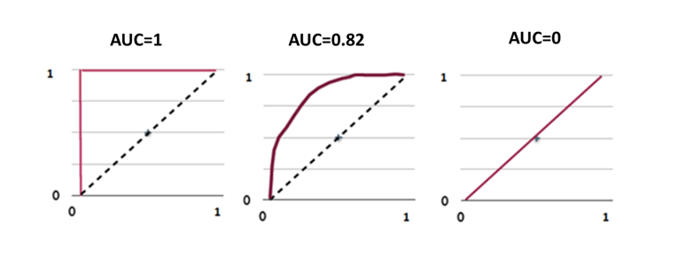
Henceforth, we can say that if area under the curve is 1 (one), then the model is perfect model.  If it is 0.82, then it is nearly good.  And if it is zero (0), then the model is not at all useful and thus we want the area under the curve to be more than 85% which depends on the data and other conditions.  For a good model, it is the possible criteria that area under the curve needs to be near to 1 (one). Lastly revising about area under the curve as follows:  First of all area under the curve (AUC) comes from ROC and ROC is created by calculating the average number of mistakes that we are making while predicting the actual true positives. Therefore, the true accuracy when compared it with our error i.e., the ROC curve and area under the ROC curve is need to be near to 1 (one) for a good model.

ROC and AUC Calculation

Building a Logistic Regression Model

Product_slaes <- read.csv("C:/Users/narahari/Desktop/Product_sales.csv")
prod_sales_Logit_model<- glm(Bought ~ Age, family=binomial,data=Product_slaes)
summary(prod_sales_Logit_model)

## 
## Call:
## glm(formula = Bought ~ Age, family = binomial, data = Product_slaes)
## 
## Deviance Residuals: 
##     Min       1Q   Median       3Q      Max  
## -3.6922  -0.1645  -0.0619   0.1246   3.5378  
## 
## Coefficients:
##             Estimate Std. Error z value Pr(>|z|)    
## (Intercept) -6.90975    0.72755  -9.497   <2e-16 ***
## Age          0.21786    0.02091  10.418   <2e-16 ***
## ---
## Signif. codes:  0 '***' 0.001 '**' 0.01 '*' 0.05 '.' 0.1 ' ' 1
## 
## (Dispersion parameter for binomial family taken to be 1)
## 
##     Null deviance: 640.425  on 466  degrees of freedom
## Residual deviance:  95.015  on 465  degrees of freedom
## AIC: 99.015
## 
## Number of Fisher Scoring iterations: 7

Now let us see how to calculate ROC and AUC (area under the curve).  We will consider the dataset product_sales_data which is the same dataset that we have used in logistic regression and in that dataset, there are two variables called age versus buy. . By building the logistic model we have predicted based on age i.e., whether a person will buy the product or not .  We already have the accuracy and confusion matrix, but we need to see is the overall area under the curve and ROC curve. For ROC curve, we need the predicted probabilities and the input of ROC curve is predicted probabilities versus actual model values.  For storing that we need to use ROC function.  For running ROC function, there is a library called pROC, thus it need to be install which attaches few other libraries.  Using pROC, we can run the ROC function. Thus ROC is created and now we just need to plot ROC. As we have discussed, the ROC curve need to be as much away from the actual line as possible.  The area under the curve is already given as 98.3%.

auc(roccurve)

Area under the curve: 0.983

auc(prod_sales_Logit_model$y, predicted_prob)

Area under the curve: 0.983 . In fact we have directly use the AUC function i.e., the area under the curve is 98.3%, or even when we write it directly without ROC curve and with predicted verses actual values or vice versa then we can get the area under the curve (AUC). . Now lets do this for a different dataset. . Now let’s do this for a little complicated data thats is fibre bits model. . The area under the curve (AUC) and ROC curve are calculated at every level of sensitivity and specificity. . So how many mistakes on an average we are doing for every model which can be calculated. . If we built multiple models then it will take some time to calculate area under the curve (AUC). . Now applying this on Fibre bits model. . First we are finding out the predicted probabilities for fibre bits model. . Then we will use ROC function and store it on ROC curve. . As we discussed earlier, it will take some time to actually create the ROC curve. . Once it created we can plot it quickly. . Thus ROC will be considered at every threshold value like what sensitivity is and what is specificity . . When threshold values will be 0.1, 0.2, 0.3, 0.4, etc. then there are many permutations and combinations that threshold will go through and find the values of predicted probabilities, specificity and sensitivity values, and finally store them in the ROC curve. . Then once this is done, we can save it in ROC and see the AUC curve.

Code – ROC Calculation

library(pROC)

## Warning: package 'pROC' was built under R version 3.3.2

## Type 'citation("pROC")' for a citation.

## 
## Attaching package: 'pROC'

## The following objects are masked from 'package:stats':
## 
##     cov, smooth, var

predicted_prob<-predict(prod_sales_Logit_model,type="response")
roccurve <- roc(prod_sales_Logit_model$y, predicted_prob)
plot(roccurve)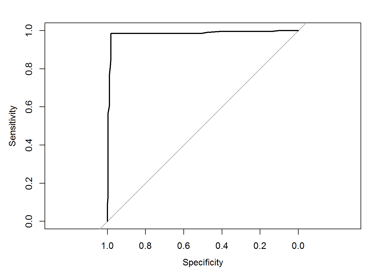

## 
## Call:
## roc.default(response = prod_sales_Logit_model$y, predictor = predicted_prob)
## 
## Data: predicted_prob in 262 controls (prod_sales_Logit_model$y 0) < 205 cases (prod_sales_Logit_model$y 1).
## Area under the curve: 0.983

Code – AUC Calculation

auc(roccurve)

## Area under the curve: 0.983

Or

auc(prod_sales_Logit_model$y, predicted_prob)

## Area under the curve: 0.983

Code-ROC from Fiberbits Model

predicted_prob<-predict(Fiberbits_model_1,type="response")
roccurve <- roc(Fiberbits_model_1$y, predicted_prob)
plot(roccurve)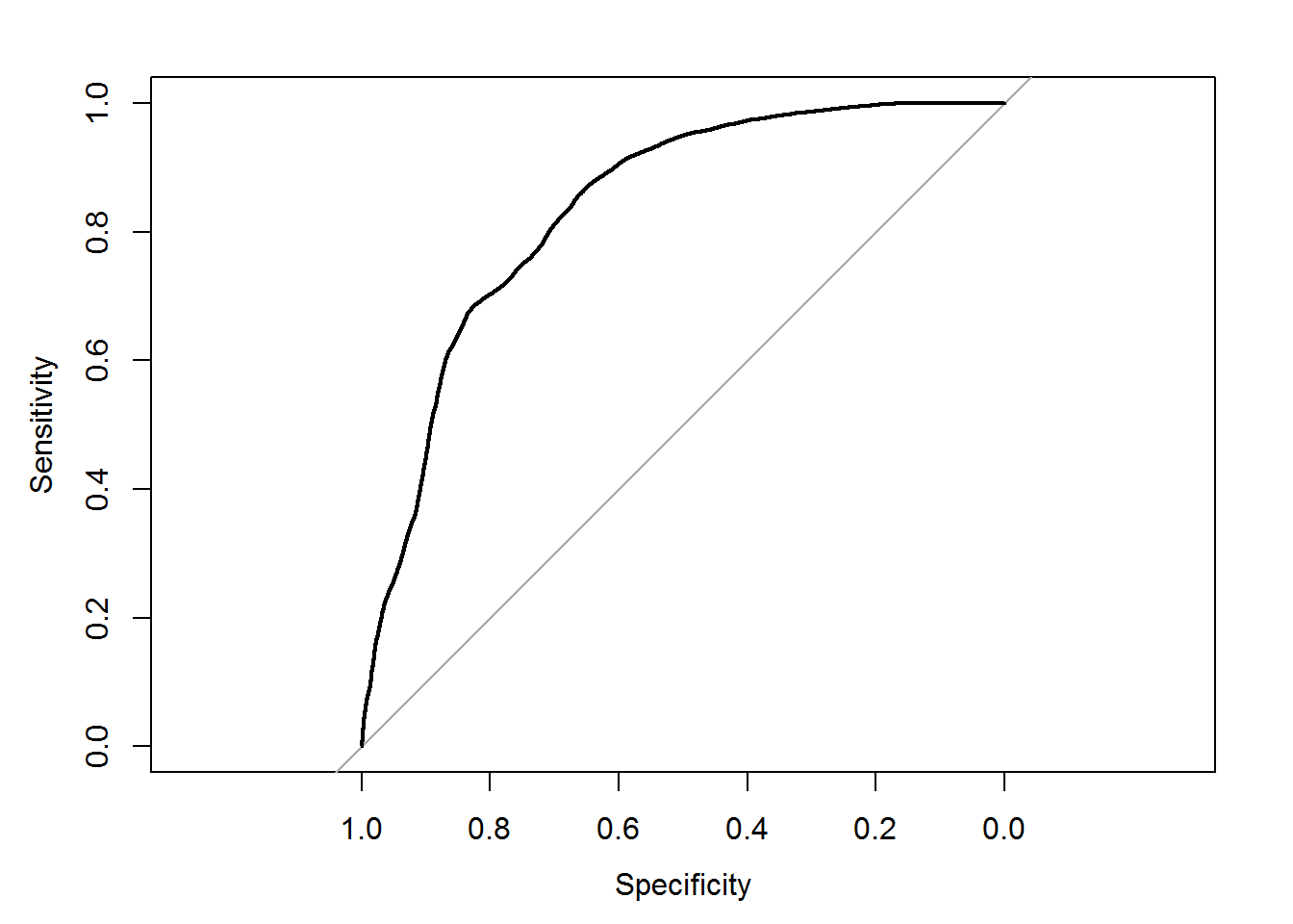

## 
## Call:
## roc.default(response = Fiberbits_model_1$y, predictor = predicted_prob)
## 
## Data: predicted_prob in 42141 controls (Fiberbits_model_1$y 0) < 57859 cases (Fiberbits_model_1$y 1).
## Area under the curve: 0.835

Code-AUC of Fiberbits Model

auc(roccurve)

## Area under the curve: 0.835

What is a best model? How to build?

Now what a best model is. Till now according to our understanding, the model with highest accuracy and least error is the best model. Or the model that uses maximum information available in the given data is the best model. Or the model that has minimum squared error; if it is the regression case, then the prediction need to be as near as possible to the actual values. Or the model that captures all the hidden patterns in the data is the actual good model. Or the model produces best predictions results is the best model. Imagine that we have multiple models; model-1, model-2 and model-3 on the same data using different techniques that how to choose the best model. Now we need to be little careful here about the error on the training data is not a good measure of performance on the future data. The future data is the unknown data model which is built on certain given dataset. A good model is measuring its goodness of fit on the given data set. . Now this might not be a good measure at all the time. This statement comprehends that the data set we use for model building is the training dataset and till now we have been looking at training error only. We actually need to look at some other error also called test error or hold out sample error. Now the questions are what exactly the test error is, what test data set is, what test error is, what hold – out dataset is and what hold-out error is. What exactly the most accurate model is, how do we see it and what is the different measure after considering apart from the training error. Let us look at an example of the most accurate model and where exactly it fails in satisfying the condition of test error.

The Most Accurate Model

Let us try to fit the best model on Fibre bits data.  We just want to predict the active customer based on remaining variables. Initially let’s start with a simple model that we are trying to fit and then see its accuracy.

library(rpart)

## Warning: package 'rpart' was built under R version 3.3.2

Fiber_bits_tree1<-rpart(active_cust~., method="class", control=rpart.control(minsplit=30, cp=0.01), data=Fiberbits)
        Fbits_pred1<-predict(Fiber_bits_tree1, type="class")
    conf_matrix1<-table(Fbits_pred1,Fiberbits$active_cust)
    accuracy1<-(conf_matrix1[1,1]+conf_matrix1[2,2])/(sum(conf_matrix1))
    accuracy1

## [1] 0.84629

    ## [1] 0.84629

The accuracy of this model is around 84%. For the 2nd model of the same dataset, let us consider the min split value as 5 and see the accuracy of this model.

 Fiber_bits_tree2<-rpart(active_cust~., method="class", control=rpart.control(minsplit=5, cp=0.000001), data=Fiberbits)
    Fbits_pred2<-predict(Fiber_bits_tree2, type="class")
    conf_matrix2<-table(Fbits_pred2,Fiberbits$active_cust)
    accuracy2<-(conf_matrix2[1,1]+conf_matrix2[2,2])/(sum(conf_matrix2))
    accuracy2

## [1] 0.95063

    ## [1] 0.95063

The accuracy of the second model is 95%. Earlier we built a model for which we got the accuracy as 84%. We changed some of the parameters and we got an accuracy of 95%. Is the accuracy of model 2, the accuracy of the final model? Is it a true representative of the model prediction power?  May be if we change the parameters a bit more, i.e., change the minimum split value or the complexity parameter, then definitely we will get much more accuracy . So what exactly defines the accuracy of a model?  The data on which we build the model is called the training dataset. . We need to find out whether training data is the final indicator, for finding out the overall model accuracy. Whether the model with 95% accuracy, the best model that we can produce.

LAB: The Most Accurate Model

• Data: Fiberbits/Fiberbits.csv
• Build a decision tree to predict active_user
• What is the accuracy of your model?
• Grow the tree as much as you can and achieve 95% accuracy.

Solution

• Model-1

library(rpart)
library(rpart.plot)

## Warning: package 'rpart.plot' was built under R version 3.3.2

Fiber_bits_tree1<-rpart(active_cust~., method="class", control=rpart.control(minsplit=30, cp=0.01), data=Fiberbits)
prp(Fiber_bits_tree1)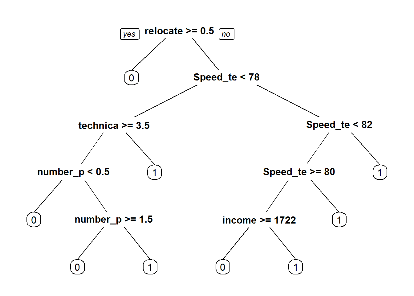

Fbits_pred1<-predict(Fiber_bits_tree1, type="class")
conf_matrix1<-table(Fbits_pred1,Fiberbits$active_cust)
accuracy1<-(conf_matrix1[1,1]+conf_matrix1[2,2])/(sum(conf_matrix1))
accuracy1

## [1] 0.84629

• Model-2

Fiber_bits_tree2<-rpart(active_cust~., method="class", control=rpart.control(minsplit=5, cp=0.000001), data=Fiberbits)
Fbits_pred2<-predict(Fiber_bits_tree2, type="class")
conf_matrix2<-table(Fbits_pred2,Fiberbits$active_cust)
accuracy2<-(conf_matrix2[1,1]+conf_matrix2[2,2])/(sum(conf_matrix2))
accuracy2

## [1] 0.95063

Different Type of Datasets and Errors

In reality there are two different types of datasets and two different types of the errors while Observing from the model building point of view . . Till now whatever the data which we have been using is the input data for building the model called the training dataset and the error that we have been calculating is the training error. For the best model, we have accuracy of 95% and we have an error of 5%. Now the question is this model really good ? By observing the model, we concludes that affirmatively, it is a really good model. . The error on the training data is known as training error. . The low error rate on the training data might not always mean that the model is good. The accuracy on training data might not be always indicative of a really good model. . Here what really matters is how the model going to perform on the unknown dataset or the test dataset or the new dataset. . Statement comprehends that we need to find out a way to get an idea of the error rate on the unknown dataset or the test dataset. One easy way is to just keep a part of the dataset and don’t use it for building the model. . For example the 80% of the data is taken and used as the training set and remaining 20% of the data is used as the testing set. But still we built the model on 80% of the data and then find the accuracy on rest of the 20% of the data which is called it as hold-out data or test data. . If the model is still doing and good prediction job on the unknown data or the out of time data or the validation data and it is still as accurate as training data, then we can be certain of the true predictive power of the model. There are two types of datasets and two types of errors. One is training dataset i.e., the actual model input data. . And the other one is test dataset which is the unknown dataset or the validation dataset that we keep aside to test our model. . The method is like once we build the model on training data, then we test it on the test dataset and then it gives the final accuracy of the final model which builds on the training dataset. Generally, we might not have all these two datasets at beginning of any problem. . All the time we will have the training dataset or sometimes we will have training + test dataset. When we will be having only training dataset then at that time we can take 90% of the available data as training data and rest 10% of the data validate as validation dataset. Validation is nothing but the substitute to test dataset or it’s a temporary test dataset. . Since we don’t have the test dataset, we have created the validation dataset. Sometimes it is created with the rule of 70% training and 30% validation or even with 80% training and 20% validation. . Hence we will build a model on the training data set, see its accuracy and the error rate. . Then this model is tested on the test data or the validation data to find its accuracy and error rate on the test data. The error rate from training data is called training error and the error rate from test data is called testing error. There are two types of errors. . One is training error which is the error that we have been calculating till now i.e., the error on the training dataset. It is also known as in-time error, the error on the input data, the error on the known data, or the error on the dataset that is used for building the model. It can be reduced while building the model and we have been trying to reduce the error as much as possible while building the model. . Even we have been trying for many iteration in building the model to reduce the error or the training error.  The second one is the test error and this error which really matters and it is also known as out of time error on the unknown dataset or the new dataset. If a model is really doing well on training dataset then it should be well on test dataset too. If it is not doing well then that is not really best model, we need to re-built or re-calculated . . Generally a good model should perform well on both the test and training data. Thus we will build the model on training dataset hence the training error will be less and then we will be validating it on test data hence the test error will be less. . But both of them should be as close to zero as possible. If a model is good on training data and it is not doing well on test data, then that is called the problem of over fitting. Let us see what exactly the problem of over fitting is.

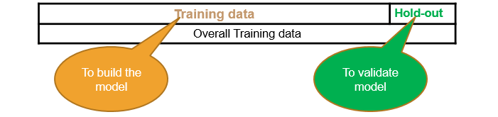
Two Types of Datasets

• There are two types of datasets
• Training set: This is used in model building. The input data
• Test set: The unknown dataset. This dataset is gives the accuracy of the final model
• We may not have access to these two datasets for all machine learning problems. In some cases, we can take 90% of the available data and use it as training data and rest 10% can be treated as validation data
• Validation set: This dataset kept aside for model validation and selection. This is a temporary subsite to test dataset. It is not third type of data
• We create the validation data with the hope that the error rate on validation data will give us some basic idea on the test error

The Problem of Over Fitting

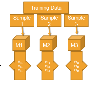
If a model is working good on the training data but not doing well on the test data then it may be due to over fitting.  Most of the models suffer from a problem called over fitting.  What exactly is over fitting? Over fitting is the result of putting too much effort in building a model for reducing the error rate or increasing the accuracy. What is the problem of the over fitting? In search of best model on the given training data we add as many predictors as possible. We add so many interaction terms, transformations, derived variables, indicator variables, dummy variables, etc. just to reduce the error. So we complicate the model knowing or unknowingly. To create a perfect model, we keep on growing the tree which makes the tree more complicated. By doing this we can reduce the training error or the error on the training data, but is this enough.  Finally we end up with an very high complicated model where the training error is less . Will this be a perfect model? Have we calculated the test error? That is, while building a model, if we just try to reduce the training error but not consider the test error then this may led to the problem called over fitting.  Let’s consider a training data which is divides into 3 random samples, sample-1, sample-2 and sample-3.  If we try to build a model on sample-1, then we get few parameters, say theta1, theta2, and theta3. Now if we build a model on sample-2, the parameter or result should be similar to that of sample-1 as these two are random samples, both belonging to the same training data set.  But if we try to build a model for sample-2, which works perfectly for the sample, so that there are no errors in the model for that sample, then the results of model 1 and model 2 may differ. We can also say that the model 2 is over fitted. This phenomena is called over fitting. . Same goes with model 3 as well.  The model is made so complicated that it becomes very sensitive to minimal changes in the dataset.  Even a small change in the value or input can affect the model. . So if the model tries to reduce the training error without even considering the test error, then this may lead to over fitting. . The over fitted model tries to fit irrelevant characteristics in the data, to increase the accuracy of the model. . Even if there is accuracy in the model, we still try to push it further and increase the accuracy to reduce the error rate which results in over fitting.  Generally an over fit model works really well on training data, but fails when it comes to test data. We even try to fit noise in the data which makes the model more complicated and resulting into over fitting.  A model needs to be a simpler one. It is ok if there are some training errors, but it should work fine with the test data as well.  Over fit model will be having a lot of variance. Even a slight change in the data may change the whole model completely.

• The model is made really complicated, that it is very sensitive to minimal changes
• By complicating the model the variance of the parameters estimates inflates
• Model tries to fit the irrelevant characteristics in the data
• Over fitting
• The model is super good on training data but not so good on test data
• We fit the model for the noise in the data
• Less training error, high testing error
• The model is over complicated with too many predictors
• Model need to be simplified
• A model with lot of variance

model with huge variance

Let us see an example of an over fitted model with huge variance. Let us consider the fibre bits data and we divide it into two parts. The dimension of the fibre bits data is 100000 observations and 9 variables.  We can consider first 90,000(ninety thousand) observations as training data and the remaining 10,000 observations as test data or validation data.

  fiber_bits_train<-Fiberbits[1:90000,]
    fiber_bits_validation<-Fiberbits[90001:100000,]

• Lets built the best model on the training dataset.

  Fiber_bits_tree3<-rpart(active_cust~., method="class", control=rpart.control(minsplit=5, cp=0.000001), data=fiber_bits_train)
    Fbits_pred3<-predict(Fiber_bits_tree3, type="class")
    conf_matrix3<-table(Fbits_pred3,fiber_bits_train$active_cust)
    accuracy3<-(conf_matrix3[1,1]+conf_matrix3[2,2])/(sum(conf_matrix3))
    accuracy3

## [1] 0.9524889

    ## [1] 0.9524889

. Here we have chosen the control parameters in such a way that, we will get the best model on the training data with least amount of error, or high accuracy rate. . We can see that the accuracy of the model for training data is 95%. . Is this the best model? . We can verify this by applying the same model on the fibre bits validation data. . For verifying the model on the validation data, we need to build a confusion matrix for it. . The confusion matrix doesn’t show much good results for the validation data.

  fiber_bits_validation$pred <- predict(Fiber_bits_tree3, fiber_bits_validation,type="class")
    
    conf_matrix_val<-table(fiber_bits_validation$pred,fiber_bits_validation$active_cust)
    accuracy_val<-(conf_matrix_val[1,1]+conf_matrix_val[2,2])/(sum(conf_matrix_val))
    accuracy_val

## [1] 0.7116

    ## [1] 0.7116

The accuracy for the validation data is 71% . The accuracy of the model on training data is 95% whereas the accuracy for validation data is 71%. So this is the typical example of over fitting. The model we built works well on the training data, giving maximum accuracy but if the same model is applied on a test data or a similar dataset, we wont get better accuracy, i.e., the variance of this model is very high. This phenomenon is called over fitting. We have over fit the model to get maximum accuracy on the training data. ### LAB: Model with huge Variance

• Data: Fiberbits/Fiberbits.csv
• Take initial 90% of the data. Consider it as training data. Keep the final 10% of the records for validation.
• Build the best model(5% error) model on training data.
• Use the validation data to verify the error rate. Is the error rate on the training data and validation data same?

Solution

fiber_bits_train<-Fiberbits[1:90000,]
fiber_bits_validation<-Fiberbits[90001:100000,]

Model on trining data

Fiber_bits_tree3<-rpart(active_cust~., method="class", control=rpart.control(minsplit=5, cp=0.000001), data=fiber_bits_train)
Fbits_pred3<-predict(Fiber_bits_tree3, type="class")
conf_matrix3<-table(Fbits_pred3,fiber_bits_train$active_cust)
accuracy3<-(conf_matrix3[1,1]+conf_matrix3[2,2])/(sum(conf_matrix3))
accuracy3

## [1] 0.9524889

Validation Accuracy

fiber_bits_validation$pred <- predict(Fiber_bits_tree3, fiber_bits_validation,type="class")

conf_matrix_val<-table(fiber_bits_validation$pred,fiber_bits_validation$active_cust)
accuracy_val<-(conf_matrix_val[1,1]+conf_matrix_val[2,2])/(sum(conf_matrix_val))
accuracy_val

## [1] 0.7116

Error rate on validation data is more than the training data error.

The Problem of Under-fitting

We saw that, if a model works very well on the training data but fails to give good accuracy on the test data or some similar data, then this model is said to be over fitted.The model which are over fitted are very complicated model .  So now the question is, will an simpler model will give good results? Not really, if a model is over simplified then we might not be capturing all the data. Suppose if we really require 20 variables and we are using only the 10 variables then we have a chance to loose out the real good information that is present in the dataset itself. If we don’t do enough research and feature re-engineering, then we cannot come up the best fit model on the dataset, which is given to us. If the model for a data set is really simple, then the training error itself will be really high and the test error will be higher. Our model need to be complicated enough to capture all the information that is present in the data. By over simplifying the model, we are not utilising all the information present in the data. We are missing some important patterns or losing the relevant information in the data which leads to a problem called under fitting. For measuring the error rate we have various measures like confusion matrix, accuracy, etc. These measures are tried on the training data first, so, if the training error itself is 30% or the accuracy is 60%, then we can conclude that the model is not a good one . Such models which are very much simplified, which are biased within itself and are very much away from the target or the final result that we are trying to predict, are called under fitted models. Over simplification is not a solution for a good model. We need to do proper research on the data and make use of all relevant information to build a proper model. We might have to add some more variables to increase the accuracy of the model. An over fitted model will be having huge variance, whereas, under fitted model will be with a lot of bias. – Under fitting – A model that is too simple – A mode with a scope for improvement – A model with lot of bias

LAB: Model with huge Bias

• Lets simplify the model.
• Take the high variance model and prune it.
• Make it as simple as possible.
• Find the training error and validation error.

Solution

• Simple Model

Fiber_bits_tree4<-rpart(active_cust~., method="class", control=rpart.control(minsplit=30, cp=0.25), data=fiber_bits_train)
prp(Fiber_bits_tree4)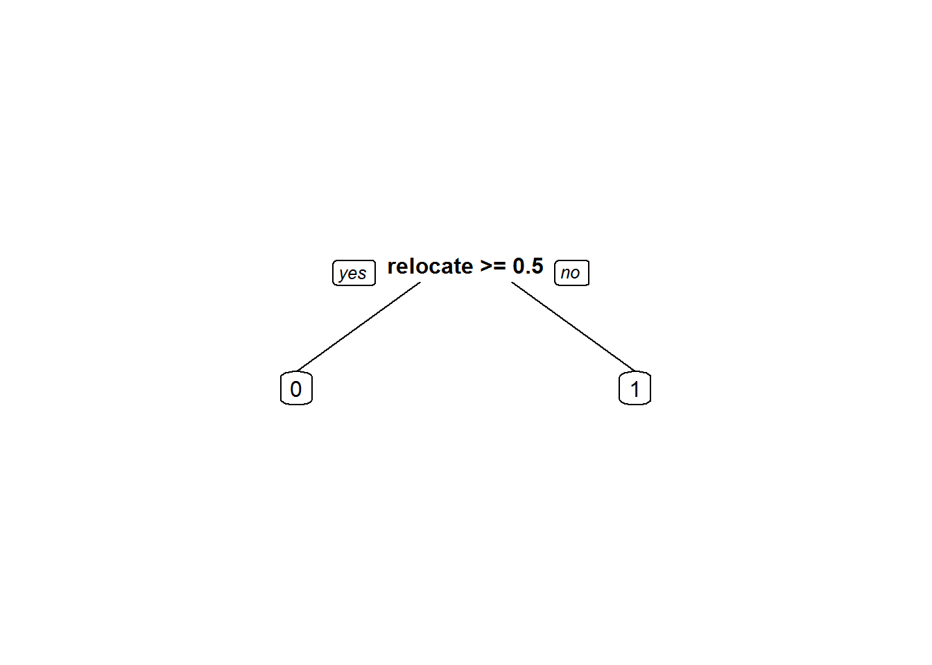

Fbits_pred4<-predict(Fiber_bits_tree4, type="class")
conf_matrix4<-table(Fbits_pred4,fiber_bits_train$active_cust)
conf_matrix4

##            
## Fbits_pred4     0     1
##           0 11209   921
##           1 25004 52866

accuracy4<-(conf_matrix4[1,1]+conf_matrix4[2,2])/(sum(conf_matrix4))
accuracy4

## [1] 0.7119444

• Validation accuracy

fiber_bits_validation$pred1 <- predict(Fiber_bits_tree4, fiber_bits_validation,type="class")

conf_matrix_val1<-table(fiber_bits_validation$pred1,fiber_bits_validation$active_cust)
accuracy_val1<-(conf_matrix_val1[1,1]+conf_matrix_val1[2,2])/(sum(conf_matrix_val1))
accuracy_val1

## [1] 0.4224

Model Bias and Variance

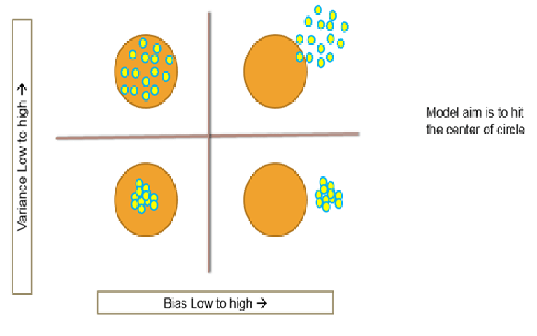
Let us do a quick recap on models with huge bias and huge variance. . As we saw earlier, over fitted models will have low bias, that means we don’t lose any relevant information which is available in the training dataset. But here the model will have huge variance, because we try to over fit every variation within the training sample, due to which we end up building the best model just for that dataset. Even a small change in the dataset will create huge variance in the model. . Hence we can say that over fitted model will have low training error and low bias but high testing error. This can be a very unstable model with high variance, and the coefficients of the model tend to change with small changes in the data. . This is called over fitting of the model, with huge variance. Under fitting means huge bias and low variance. There is already certain bias in building the model, where the training data error itself is high, so the testing error will definitely be more than training error. It’s a stable model with low variance. The coefficient of the model doesn’t change much with changes in the data,but there is no use of it because the training error in itself is really high . . Let us understand the variance and bias in an easy way. Look at these four circles in the diagrams. Here our aim is to hit the centre of the circle i.e., using the model we want to predict centre of the circle. If we are hitting all of them at the centre, as we can see in the bottom left circle, then this is the model with low bias and low variance. Now if we consider the bottom right model, we can see that the model has very high bias but low variance, which means, all the points that we are hitting are closer to each other, but they are not hitting at the centre.  If we see the top left model, we can see that it is having low bias as most of the points are hitting near the centre, but very high variance as none of the points are closer to each other. – Now the top right model, as we can see, has high bias as none of the points are near the centre and high variance as the points are not closer to each other. So from the above observations we can say that the bottom left model is the best model out of all 4 models as the bias and variance both are very less in this model. In fact we can prove that the overall error is nothing but, sum of irreducible error, bias and variance . The overall error that any model will make is nothing but Bias2 + Variance+ irreducible error i.e.,the random error or the error that is present as it is. This is called Bias-Variance Decomposition. . A good model needs to have low bias as well as low variance. So our major effort is choosing the best model or the optimal model which will have low variance and low bias i.e., the best fitted model with optimal complexity. . For a good model we neither over fit nor under fit. We need to choose the right model complexity for an optimal model. – Over fitting – Low Bias with High Variance – Low training error – ‘Low Bias’ – High testing error – Unstable model – ‘High Variance’ – The coefficients of the model change with small changes in the data – Under fitting – High Bias with low Variance – High training error – ‘high Bias’ – testing error almost equal to training error – Stable model – ‘Low Variance’ – The coefficients of the model doesn’t change with small changes in the data

The Bias-Variance Decomposition

Overall Model Squared Error = Irreducible Error + (Bias^2) + Variance

Bias-Variance Decomposition

• Overall Model Squared Error = Irreducible Error + (Bias^2) + Variance
• Overall error is made by bias and variance together
• High bias low variance, Low bias and high variance, both are bad for the overall accuracy of the model
• A good model need to have low bias and low variance or at least an optimal where both of them are jointly low
• How to choose such optimal model. How to choose that optimal model complexity

Choosing optimal model-Bias Variance Tradeoff

Bias Variance Tradeoff

. How do we choose the best model? . As we saw earlier, the overall error is sum of irreducible error,bias and variance. So let us see how we consider the bias variance trade off and then finally choose the best model.

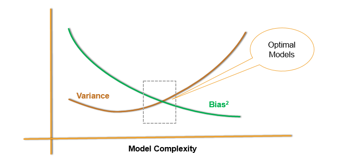
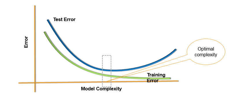
From the plot, we can see that, as the model complexity increases the bias decreases i.e., as the complexity of model increases, the bias decreases and as the model becomes simpler the bias increases. . We can also observe that, as the model complexity increases, initially the variance reduces but later on as the model complexity becomes very high, the variance of the model increases. Hence we can say that the model which come in this region, i.e., having less bias value and less variance, are considered to be the optimal model. If there are, say 20 variables in the data and if the 10th variable come in line with the optimal region, i.e., less bias value and less variance, then the model with those 10 variables will be the best model. If we consider all 20 variables, the bias value will be less and the variance will be high i.e., the model will be a over fitted model. On other hand if we consider only 5 variable, then bias value will be high and variance will be low, which gives an under fitted model. So an optimal model is the one with low bias and low variance values. There is one more point of view to this.

Test and Training Error

Here we can see, as model complexity increases, the training error reduces i.e., if we increase the complexity, we tend to fit the model for all the patterns in the data hence reducing the training error. But If we keep on Increasing the complexity of the model, the model will be over fitted due to which the test error will also increase. . If we don’t have enough complexity then both training error and test error will be high. Here if we consider 20 variables in the dataset then considering all 20 variables will reduce the training data but increase the test data. If we consider just 5 variables then there is a possibility that both training and test error will be high. But if we consider 10 variables, which comes in the centre, both training error and the test error will be less. This will give the optimal model for our data.

Choosing optimal model-Bias Variance Tradeoff

Unfortunately there is no actual significant method or metrics that will tell us the best model complexity to be considered for an optimal model, if this the given model or there are X number of datasets and then choosing these Y parameter will given an optimal solution no there are no such method or rules. The training error is not a good estimate of the final test error. We are not sure whether we are over complicating the model or over simplifying the model. There is always a bias-variance trade off and the model complexity or the number of parameters in the model that we need to choose to get an optimal model. . How do we choose the right model, the number of parameters, etc. so that we can do the bias-variance tradeoff which can reduce the training and testing error? What is the best model we can fit on a given data? . How do we choose the optimal model complexity? For this we can use various techniques like cross validation methods, boot strapping and bagging which helps us in finding the training error, test error and final accuracy of the model, etc. so that we can choose the best model and best complexity for the given dataset.

Bias Variance Tradeoff

Test and Training Error

Choosing Optimal Model

• Unfortunately
• There is no scientific method of choosing optimal model complexity that gives minimum test error.
• Training error is not a good estimate of the test error.
• There is always bias-variance tradeoff in choosing the appropriate complexity of the model.
• We can use cross validation methods, boot strapping and bagging to choose the optimal and consistent model

Holdout Data Cross Validation

Taking hold out data or cross validation is one of the best way in finding out the actual error present in the model. As we know, the training error doesn’t really give us the original error in the model, i.e., we cannot make out whether the model is over fit or under fit. In such cases, cross validation really gives us an idea on the final accuracy of the model using which we can choose the model complexity and build a better model . What we do is, we take the out of time data or we hold out some data i.e., out of overall training data we take, let’s say 80% as training data and keep 20% as hold out data. . We try to build a model on the 80% of the training data and check the accuracy of the model on the hold out data . We can also consider the split as 90%:10% or 70%:30%.  Here the model is built on the training data and it is tested on the hold out data which acts as the test data for training data from which we get the testing error. . If the training error and testing error is similar then at least one thing is sure that we did not over fit the model on the training data. This technique is called as cross validation or hold out sample data validation, which is one of the most widely used methods to find out the accuracy of the model that we have built.

• The best solution is out of time validation. Or the testing error should be given high priority over the training error.
• A model that is performing good on training data and equally good on testing is preferred.
• We may not have the test data always. How do we estimate test error?
• We take the part of the data as training and keep aside some potion for validation. May be 80%-20% or 90%-10%
• Data splitting is a very basic intuitive method

LAB: Holdout Data Cross Validation

• Data: Fiberbits/Fiberbits.csv
• Take a random sample with 80% data as training sample
• Use rest 20% as holdout sample.
• Build a model on 80% of the data. Try to validate it on holdout sample.
• Try to increase or reduce the complexity and choose the best model that performs well on training data as well as holdout data

Solution

• Caret is a good package for cross validation

library(caret)
sampleseed <- createDataPartition(Fiberbits$active_cust, p=0.80, list=FALSE)
train_new <- Fiberbits[sampleseed,]
hold_out <- Fiberbits[-sampleseed,]

• Model1

library(rpart)
Fiber_bits_tree5<-rpart(active_cust~., method="class", control=rpart.control(minsplit=5, cp=0.000001), data=train_new)
Fbits_pred5<-predict(Fiber_bits_tree5, type="class")

• Accuracy on Training Data

conf_matrix5<-table(Fbits_pred5,train_new$active_cust)
conf_matrix5

##            
## Fbits_pred5     0     1
##           0 31377  1654
##           1  2270 44699

accuracy5<-(conf_matrix5[1,1]+conf_matrix5[2,2])/(sum(conf_matrix5))
accuracy5

## [1] 0.95095

• Model1 Validation accuracy

hold_out$pred <- predict(Fiber_bits_tree5, hold_out, type="class")
conf_matrix_val<-table(hold_out$pred,hold_out$active_cust)
conf_matrix_val

##    
##         0     1
##   0  6975  1346
##   1  1519 10160

accuracy_val<-(conf_matrix_val[1,1]+conf_matrix_val[2,2])/(sum(conf_matrix_val))
accuracy_val

## [1] 0.85675

• Model2

Fiber_bits_tree5<-rpart(active_cust~., method="class", control=rpart.control(minsplit=30, cp=0.05), data=train_new)
Fbits_pred5<-predict(Fiber_bits_tree5, type="class")
conf_matrix5<-table(Fbits_pred5,train_new$active_cust)

• Accuracy on Training Data

accuracy5<-(conf_matrix5[1,1]+conf_matrix5[2,2])/(sum(conf_matrix5))
accuracy5

## [1] 0.78885

• Model2 Validation accuracy

hold_out$pred <- predict(Fiber_bits_tree5, hold_out,type="class")
conf_matrix_val<-table(hold_out$pred,hold_out$active_cust)
accuracy_val<-(conf_matrix_val[1,1]+conf_matrix_val[2,2])/(sum(conf_matrix_val))
accuracy_val

## [1] 0.7898

• Model3

Fiber_bits_tree5<-rpart(active_cust~., method="class", control=rpart.control(minsplit=30, cp=0.001), data=train_new)
Fbits_pred5<-predict(Fiber_bits_tree5, type="class")
conf_matrix5<-table(Fbits_pred5,train_new$active_cust)

• Accuracy on Training Data

accuracy5<-(conf_matrix5[1,1]+conf_matrix5[2,2])/(sum(conf_matrix5))
accuracy5

## [1] 0.8695625

• Model3 Validation accuracy

hold_out$pred <- predict(Fiber_bits_tree5, hold_out,type="class")
conf_matrix_val<-table(hold_out$pred,hold_out$active_cust)
accuracy_val<-(conf_matrix_val[1,1]+conf_matrix_val[2,2])/(sum(conf_matrix_val))
accuracy_val

## [1] 0.8658

Ten-fold Cross – Validation

We saw the example of cross validation, where we took the overall training data, we took 80% of it and used it as training data and remaining 20% as the hold out data.  We did this process once. If we do it ten times then it is called ten fold cross validation . Let us see how it is done . We first divide the whole dataset into ten parts randomly, use 9 parts as training data and the tenth part as holdout data . We have to build 10 models so we repeat the whole process 10 times. After Building 10 models, we find the average error of 10 holdout samples and this really gives us the actual training error. Even smallest error which were occurring earlier can be reduced used the 10 fold cross validation. So how it is done? 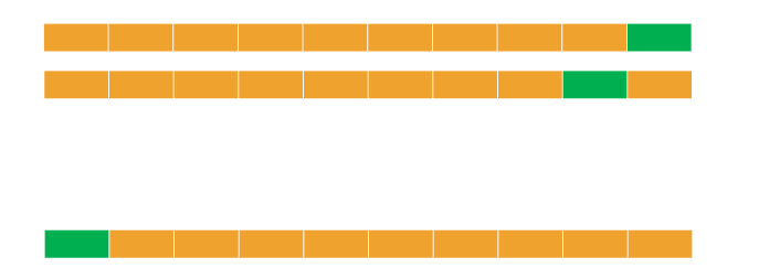Let us consider a dataset and divide into 10 sample dataset. For the 1st model, from 1 to 9 samples will be the training data and the 10th sample will be the holdout data. The model can be build for the training data and can be tested on the hold out data. . For the 2nd model all the samples except the 9th sample will be considered as the training data and the 9th sample will be the holdout data. . Similarly the remaining 8 models are formed. For the 10th model, the 1st sample will be the holdout data and the remaining 9 samples will be the training data. This is how we do k fold cross validation. A 10 fold validation will have 10 errors for each model, and using the average of these values, we get the overall error and accuracy of the model that we build. We can generalise this validation technique as the k-fold validation . As we saw in a 10 fold validation, the data was divided into 10 parts, so in a k- fold validation the data will be divided into k parts. Among the k parts, one of them will be considered as the test data and the remaining parts or folds will be treated as training data. . If k value is 10,then it will be a 10 fold cross validation. If the k value is 5, then 80% of the data will be considered for training and the remaining 20% will be considered for testing. . The k validation is just the general form of the 10 fold cross validation .  So we can say that, for a k fold validation, there will be k models and the average error on the hold out data gives us an estimate on the overall testing error . How do we choose the best model ? . Always choose the model that has least error and least complexity. . Always choose a model that is simple and is capturing most of the information or the model with less than average error but looks simple, which means it has least parameters. . So we can build a different model using the overall dataset with those parameters. From this we get an idea on the overall error and the complexity of the model. Then we can take the overall training dataset, use the same complexity and rebuilt the our final model. . Every time in the k fold validation, i.e., for every fold if we are getting an accuracy of 80% then the overall accuracy of the model will be 80%. Generally in k-fold cross validation, it’s better to choose k between 5 and 10, which gives 80% to 90% training data and rest of the 20% to 10% will be the holdout data respectively .

K-fold Cross Validation

• A generalization of cross validation.
• Divide the whole dataset into k equal parts
• Use kth part of the data as the holdout sample, use remaining k-1 parts of the data as training data
• Repeat this K times, build K models. The average error on holdout sample gives us an idea on the testing error
• Which model to choose?
• Choose the model with least error and least complexity
• Or the model with less than average error and simple (less parameters)
• Finally use complete data and build a model with the chosen number of parameters
• Note: Its better to choose K between 5 to 10. Which gives 80% to 90% training data and rest 20% to 10% is holdout data

LAB – K-fold Cross Validation

• Build a tree model on the fiber bits data.
• Try to build the best model by making all the possible adjustments to the parameters.
• What is the accuracy of the above model?
• Perform 10 -fold cross validation. What is the final accuracy?
• Perform 20 -fold cross validation. What is the final accuracy?
• What can be the expected accuracy on the unknown dataset?

Solution

• Model on complete training data

Fiber_bits_tree3<-rpart(active_cust~., method="class", control=rpart.control(minsplit=10, cp=0.000001), data=Fiberbits)
Fbits_pred3<-predict(Fiber_bits_tree3, type="class")
conf_matrix3<-table(Fbits_pred3,Fiberbits$active_cust)
conf_matrix3

##            
## Fbits_pred3     0     1
##           0 38154  2849
##           1  3987 55010

• Accuracy on Traing Data

accuracy3<-(conf_matrix3[1,1]+conf_matrix3[2,2])/(sum(conf_matrix3))
accuracy3

## [1] 0.93164

• k-fold Cross Validation building
• K=10

library(caret)
train_dat <- trainControl(method="cv", number=10)

Need to convert the dependent variable to factor before fitting the model

Fiberbits$active_cust<-as.factor(Fiberbits$active_cust)

• Building the models on K-fold samples

library(e1071)

## Warning: package 'e1071' was built under R version 3.3.2

K_fold_tree<-train(active_cust~., method="rpart", trControl=train_dat, control=rpart.control(minsplit=10, cp=0.000001),  data=Fiberbits)
K_fold_tree$finalModel

## n= 100000 
## 
## node), split, n, loss, yval, (yprob)
##       * denotes terminal node
## 
## 1) root 100000 42141 1 (0.42141000 0.57859000)  
##   2) relocated>=0.5 12348   954 0 (0.92274052 0.07725948) *
##   3) relocated< 0.5 87652 30747 1 (0.35078492 0.64921508)  
##     6) Speed_test_result< 78.5 27517 10303 0 (0.62557692 0.37442308) *
##     7) Speed_test_result>=78.5 60135 13533 1 (0.22504365 0.77495635) *

prp(K_fold_tree$finalModel)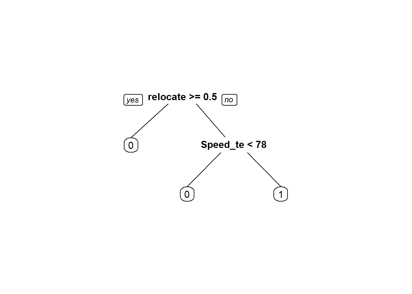

Kfold_pred<-predict(K_fold_tree)
conf_matrix6<-confusionMatrix(Kfold_pred,Fiberbits$active_cust)
conf_matrix6

## Confusion Matrix and Statistics
## 
##           Reference
## Prediction     0     1
##          0 28608 11257
##          1 13533 46602
##                                           
##                Accuracy : 0.7521          
##                  95% CI : (0.7494, 0.7548)
##     No Information Rate : 0.5786          
##     P-Value [Acc > NIR] : < 2.2e-16       
##                                           
##                   Kappa : 0.4879          
##  Mcnemar's Test P-Value : < 2.2e-16       
##                                           
##             Sensitivity : 0.6789          
##             Specificity : 0.8054          
##          Pos Pred Value : 0.7176          
##          Neg Pred Value : 0.7750          
##              Prevalence : 0.4214          
##          Detection Rate : 0.2861          
##    Detection Prevalence : 0.3987          
##       Balanced Accuracy : 0.7422          
##                                           
##        'Positive' Class : 0               
## 

• K=20

library(caret)
train_dat <- trainControl(method="cv", number=20)

Need to convert the dependent variable to factor before fitting the model

Fiberbits$active_cust<-as.factor(Fiberbits$active_cust)

Building the models on K-fold samples

library(e1071)
K_fold_tree_1<-train(active_cust~., method="rpart", trControl=train_dat, control=rpart.control(minsplit=10, cp=0.000001),  data=Fiberbits)
K_fold_tree_1$finalModel

## n= 100000 
## 
## node), split, n, loss, yval, (yprob)
##       * denotes terminal node
## 
## 1) root 100000 42141 1 (0.42141000 0.57859000)  
##   2) relocated>=0.5 12348   954 0 (0.92274052 0.07725948) *
##   3) relocated< 0.5 87652 30747 1 (0.35078492 0.64921508)  
##     6) Speed_test_result< 78.5 27517 10303 0 (0.62557692 0.37442308) *
##     7) Speed_test_result>=78.5 60135 13533 1 (0.22504365 0.77495635) *

prp(K_fold_tree_1$finalModel)

Kfold_pred<-predict(K_fold_tree_1)

Caret package has confusion matrix function

conf_matrix6_1<-confusionMatrix(Kfold_pred,Fiberbits$active_cust)
conf_matrix6_1

## Confusion Matrix and Statistics
## 
##           Reference
## Prediction     0     1
##          0 28608 11257
##          1 13533 46602
##                                           
##                Accuracy : 0.7521          
##                  95% CI : (0.7494, 0.7548)
##     No Information Rate : 0.5786          
##     P-Value [Acc > NIR] : < 2.2e-16       
##                                           
##                   Kappa : 0.4879          
##  Mcnemar's Test P-Value : < 2.2e-16       
##                                           
##             Sensitivity : 0.6789          
##             Specificity : 0.8054          
##          Pos Pred Value : 0.7176          
##          Neg Pred Value : 0.7750          
##              Prevalence : 0.4214          
##          Detection Rate : 0.2861          
##    Detection Prevalence : 0.3987          
##       Balanced Accuracy : 0.7422          
##                                           
##        'Positive' Class : 0               
## 

Bootstrap Methods

• Boot strapping is a powerful tool to get an idea on accuracy of the model and the test error
• Can estimate the likely future performance of a given modeling procedure, on new data not yet realized.
• The Algorithm
• We have a training data is of size N
• Draw random sample with replacement of size N – This gives a new dataset, it might have repeated observations, some observations might not have even appeared once.
• Create B such new datasets. These are called boot strap datasets
• Build the model on these B datasets, we can test the models on the original training dataset.

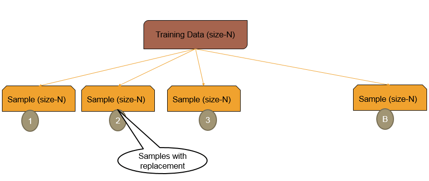
Bootstrap Example

• Example

1. We have a training data is of size 500
2. Boot Strap Data-1:

• Create a dataset of size 500. To create this dataset, draw a random point, note it down, then replace it back. Again draw another sample point. Repeat this process 500 times. This makes a dataset of size 500. Call this as Boot Strap Data-1

3. Multiple Boot Strap datasets

• Repeat the procedure in step -2 multiple times. Say 200 times. Then we have 200 Boot Strap datasets

4. We can build the models on these 200 boost strap datasets and the average error gives a good idea on overall error. We can even use the original training data as the test data for each of the models

LAB: Bootstrap Cross Validation

• Draw a boot strap sample with sufficient sample size
• Build a tree model and get an estimate on true accuracy of the model

Solution

• Draw a boot strap sample with sufficient sample size

Where number is B

train_control <- trainControl(method="boot", number=20) 

Tree model on boots straped data

Boot_Strap_model <- train(active_cust~., method="rpart", trControl= train_control, control=rpart.control(minsplit=10, cp=0.000001),  data=Fiberbits)
Boot_Strap_predictions <- predict(Boot_Strap_model)

conf_matrix7<-confusionMatrix(Boot_Strap_predictions,Fiberbits$active_cust)
conf_matrix7

## Confusion Matrix and Statistics
## 
##           Reference
## Prediction     0     1
##          0 28608 11257
##          1 13533 46602
##                                           
##                Accuracy : 0.7521          
##                  95% CI : (0.7494, 0.7548)
##     No Information Rate : 0.5786          
##     P-Value [Acc > NIR] : < 2.2e-16       
##                                           
##                   Kappa : 0.4879          
##  Mcnemar's Test P-Value : < 2.2e-16       
##                                           
##             Sensitivity : 0.6789          
##             Specificity : 0.8054          
##          Pos Pred Value : 0.7176          
##          Neg Pred Value : 0.7750          
##              Prevalence : 0.4214          
##          Detection Rate : 0.2861          
##    Detection Prevalence : 0.3987          
##       Balanced Accuracy : 0.7422          
##                                           
##        'Positive' Class : 0               
## 

References

• Hastie,Tibshirani and Friedman – The Elements of Statistical Learning (2nd edition, 2009).
• http://scott.fortmann-roe.com/docs/BiasVariance.html